
1.2.E: Exercises
- Page ID
- 157143

\( \newcommand{\vecs}[1]{\overset { \scriptstyle \rightharpoonup} {\mathbf{#1}} } \)
\( \newcommand{\vecd}[1]{\overset{-\!-\!\rightharpoonup}{\vphantom{a}\smash {#1}}} \)
\( \newcommand{\dsum}{\displaystyle\sum\limits} \)
\( \newcommand{\dint}{\displaystyle\int\limits} \)
\( \newcommand{\dlim}{\displaystyle\lim\limits} \)
\( \newcommand{\id}{\mathrm{id}}\) \( \newcommand{\Span}{\mathrm{span}}\)
( \newcommand{\kernel}{\mathrm{null}\,}\) \( \newcommand{\range}{\mathrm{range}\,}\)
\( \newcommand{\RealPart}{\mathrm{Re}}\) \( \newcommand{\ImaginaryPart}{\mathrm{Im}}\)
\( \newcommand{\Argument}{\mathrm{Arg}}\) \( \newcommand{\norm}[1]{\| #1 \|}\)
\( \newcommand{\inner}[2]{\langle #1, #2 \rangle}\)
\( \newcommand{\Span}{\mathrm{span}}\)
\( \newcommand{\id}{\mathrm{id}}\)
\( \newcommand{\Span}{\mathrm{span}}\)
\( \newcommand{\kernel}{\mathrm{null}\,}\)
\( \newcommand{\range}{\mathrm{range}\,}\)
\( \newcommand{\RealPart}{\mathrm{Re}}\)
\( \newcommand{\ImaginaryPart}{\mathrm{Im}}\)
\( \newcommand{\Argument}{\mathrm{Arg}}\)
\( \newcommand{\norm}[1]{\| #1 \|}\)
\( \newcommand{\inner}[2]{\langle #1, #2 \rangle}\)
\( \newcommand{\Span}{\mathrm{span}}\) \( \newcommand{\AA}{\unicode[.8,0]{x212B}}\)
\( \newcommand{\vectorA}[1]{\vec{#1}} % arrow\)
\( \newcommand{\vectorAt}[1]{\vec{\text{#1}}} % arrow\)
\( \newcommand{\vectorB}[1]{\overset { \scriptstyle \rightharpoonup} {\mathbf{#1}} } \)
\( \newcommand{\vectorC}[1]{\textbf{#1}} \)
\( \newcommand{\vectorD}[1]{\overrightarrow{#1}} \)
\( \newcommand{\vectorDt}[1]{\overrightarrow{\text{#1}}} \)
\( \newcommand{\vectE}[1]{\overset{-\!-\!\rightharpoonup}{\vphantom{a}\smash{\mathbf {#1}}}} \)
\( \newcommand{\vecs}[1]{\overset { \scriptstyle \rightharpoonup} {\mathbf{#1}} } \)
\(\newcommand{\longvect}{\overrightarrow}\)
\( \newcommand{\vecd}[1]{\overset{-\!-\!\rightharpoonup}{\vphantom{a}\smash {#1}}} \)
\(\newcommand{\avec}{\mathbf a}\) \(\newcommand{\bvec}{\mathbf b}\) \(\newcommand{\cvec}{\mathbf c}\) \(\newcommand{\dvec}{\mathbf d}\) \(\newcommand{\dtil}{\widetilde{\mathbf d}}\) \(\newcommand{\evec}{\mathbf e}\) \(\newcommand{\fvec}{\mathbf f}\) \(\newcommand{\nvec}{\mathbf n}\) \(\newcommand{\pvec}{\mathbf p}\) \(\newcommand{\qvec}{\mathbf q}\) \(\newcommand{\svec}{\mathbf s}\) \(\newcommand{\tvec}{\mathbf t}\) \(\newcommand{\uvec}{\mathbf u}\) \(\newcommand{\vvec}{\mathbf v}\) \(\newcommand{\wvec}{\mathbf w}\) \(\newcommand{\xvec}{\mathbf x}\) \(\newcommand{\yvec}{\mathbf y}\) \(\newcommand{\zvec}{\mathbf z}\) \(\newcommand{\rvec}{\mathbf r}\) \(\newcommand{\mvec}{\mathbf m}\) \(\newcommand{\zerovec}{\mathbf 0}\) \(\newcommand{\onevec}{\mathbf 1}\) \(\newcommand{\real}{\mathbb R}\) \(\newcommand{\twovec}[2]{\left[\begin{array}{r}#1 \\ #2 \end{array}\right]}\) \(\newcommand{\ctwovec}[2]{\left[\begin{array}{c}#1 \\ #2 \end{array}\right]}\) \(\newcommand{\threevec}[3]{\left[\begin{array}{r}#1 \\ #2 \\ #3 \end{array}\right]}\) \(\newcommand{\cthreevec}[3]{\left[\begin{array}{c}#1 \\ #2 \\ #3 \end{array}\right]}\) \(\newcommand{\fourvec}[4]{\left[\begin{array}{r}#1 \\ #2 \\ #3 \\ #4 \end{array}\right]}\) \(\newcommand{\cfourvec}[4]{\left[\begin{array}{c}#1 \\ #2 \\ #3 \\ #4 \end{array}\right]}\) \(\newcommand{\fivevec}[5]{\left[\begin{array}{r}#1 \\ #2 \\ #3 \\ #4 \\ #5 \\ \end{array}\right]}\) \(\newcommand{\cfivevec}[5]{\left[\begin{array}{c}#1 \\ #2 \\ #3 \\ #4 \\ #5 \\ \end{array}\right]}\) \(\newcommand{\mattwo}[4]{\left[\begin{array}{rr}#1 \amp #2 \\ #3 \amp #4 \\ \end{array}\right]}\) \(\newcommand{\laspan}[1]{\text{Span}\{#1\}}\) \(\newcommand{\bcal}{\cal B}\) \(\newcommand{\ccal}{\cal C}\) \(\newcommand{\scal}{\cal S}\) \(\newcommand{\wcal}{\cal W}\) \(\newcommand{\ecal}{\cal E}\) \(\newcommand{\coords}[2]{\left\{#1\right\}_{#2}}\) \(\newcommand{\gray}[1]{\color{gray}{#1}}\) \(\newcommand{\lgray}[1]{\color{lightgray}{#1}}\) \(\newcommand{\rank}{\operatorname{rank}}\) \(\newcommand{\row}{\text{Row}}\) \(\newcommand{\col}{\text{Col}}\) \(\renewcommand{\row}{\text{Row}}\) \(\newcommand{\nul}{\text{Nul}}\) \(\newcommand{\var}{\text{Var}}\) \(\newcommand{\corr}{\text{corr}}\) \(\newcommand{\len}[1]{\left|#1\right|}\) \(\newcommand{\bbar}{\overline{\bvec}}\) \(\newcommand{\bhat}{\widehat{\bvec}}\) \(\newcommand{\bperp}{\bvec^\perp}\) \(\newcommand{\xhat}{\widehat{\xvec}}\) \(\newcommand{\vhat}{\widehat{\vvec}}\) \(\newcommand{\uhat}{\widehat{\uvec}}\) \(\newcommand{\what}{\widehat{\wvec}}\) \(\newcommand{\Sighat}{\widehat{\Sigma}}\) \(\newcommand{\lt}{<}\) \(\newcommand{\gt}{>}\) \(\newcommand{\amp}{&}\) \(\definecolor{fillinmathshade}{gray}{0.9}\)1.2 Exercises
Given each pair of functions, evaluate \(f(g(x))\) and \(g(f(0))\)
| 1. \(f(x) = 4x+8, g(x) = 7-x^2\) | 2. \(f(x) = 5x+7, g(x) = 4-2x^2\) |
| 3. \(f(x) = \sqrt{x+4}, g(x) = 12-x^3\) | 4. \(f(x) = \frac{1}{x+2}, g(x) = 4x+3\) |
|
x |
\(f(x)\) |
\(g(x)\) |
|
0 |
7 |
9 |
|
1 |
6 |
5 |
|
2 |
5 |
6 |
|
3 |
8 |
2 |
|
4 |
4 |
1 |
|
5 |
0 |
8 |
|
6 |
2 |
7 |
|
7 |
1 |
3 |
|
8 |
9 |
4 |
|
9 |
3 |
0 |
Use the table of values to evaluate each expression.
| 5. \(f(g(8))\) |
| 6. \(f(g(5))\) |
| 7. \(g(f(5))\) |
| 8. \(g(f(3))\) |
| 9. \(f(f(4))\) |
| 10. \(f(f(1))\) |
| 11. \(g(g(2))\) |
| 12. \(g(g(6))\) |
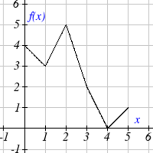
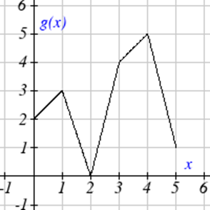
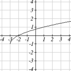
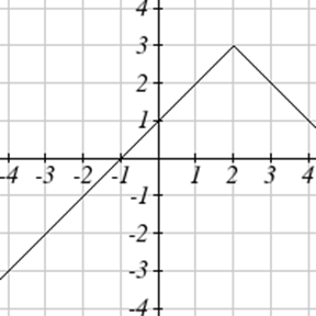
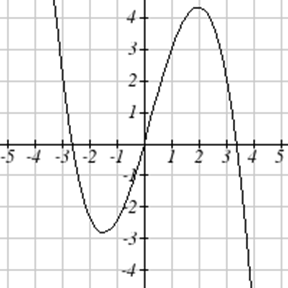
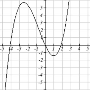
Use the graphs to evaluate the expressions below.
| 13. \(f(g(3))\) |
| 14. \(f(g(1))\) |
| 15. \(g(f(1))\) |
| 16. \(g(f(0))\) |
| 17. \(f(f(5))\) |
| 18. \(f(f(4))\) |
| 19. \(g(g(2))\) |
| 20. \(g(g(0))\) |
For each pair of functions, find \(f(g(x))\) and \(g(f(x))\). Simplify your answers.
| 21. \(f(x) = \frac{1}{x-6}, g(x) = \frac{7}{x}+6\) | 22. \(f(x) = \frac{1}{x-4}, g(x) = \frac{2}{x} + 4\) |
| 23. \(f(x) = x^2+1, g(x) = \sqrt{x+2}\) | 24. \(f(x) = \sqrt{x} + 2, g(x) = x^2 + 3\) |
| 25. \(f(x) = |x|, g(x) = 5x+1\) | 26. \(f(x) = \sqrt[3]{x}, g(x) = \frac{x+1}{x^3}\) |
If \(f(x) = x^4+6\), \(g(x) = x - 6\), and \(h(x) = \sqrt{x}\), find \(f(g(h(x)))\)
If \(f(x) = x^2+1\), \(g(x) = \frac{1}{x}\), and \(h(x) = x+3\), find \(f(g(h(x)))\)
The function \(D(p)\) gives the number of items that will be demanded when the price is \(p\). The production cost, \(C(x)\) is the cost of producing \(x\) items. To determine the cost of production when the price is $6, you would do which of the following:
- Evaluate \(D(C(6))\)
- Evaluate \(C(D(6))\)
- Solve \(D(C(x)) = 6\)
- Solve \(C(D(p)) = 6\)
The function \(A(d)\) gives the pain level on a scale of 0-10 experienced by a patient with \(d\) milligrams of a pain reduction drug in their system. The milligrams of drug in the patient’s system after \(t\) minutes is modeled by \(m(t)\). To determine when the patient will be at a pain level of 4, you would need to:
- Evaluate \(A(m(4))\)
- Evaluate \(m(A(4))\)
- Solve \(A(m(t)) = 4\)
- Solve \(m(A(d)) = 4\)
Find functions \(f(x)\) and \(g(x)\) so the given function can be expressed as \(h(x) = f(g(x))\).
| 31. \(h(x) = (x+2)^2\) | 32. \(h(x) = (x-5)^3\) |
| 33. \(h(x) = \frac{3}{x-5}\) | 34. \(h(x) = \frac{4}{(x+2)^2}\) |
| 35. \(h(x) = 3+\sqrt{x-2}\) | 36. \(h(x) = 4+\sqrt[3]{x}\) |
Sketch a graph of each function as a transformation of a toolkit function.
| 37. \(f(t) = (t+1)^2 - 3\) | 38. \(h(x) = |x-1|+4\) |
| 39. \(k(x) =(x-2)^3 -1\) | 40. \(m(t) = 3+\sqrt{t+2}\) |
| 41. \(f(x) = 4(x+1)^2 - 5\) | 42. \(g(x) = 5(x+3)^2 - 2\) |
| 43. \(h(x) = -2|x-4|+3\) | 44. \(k(x) = -3\sqrt{x} - 1\) |
Write an equation for each function graphed below.
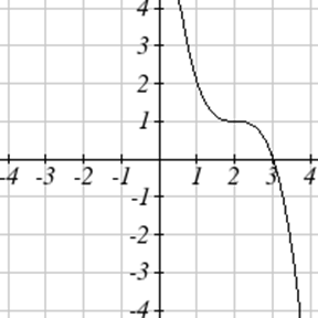
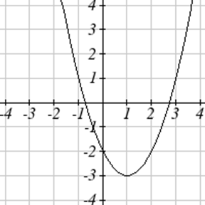
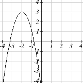
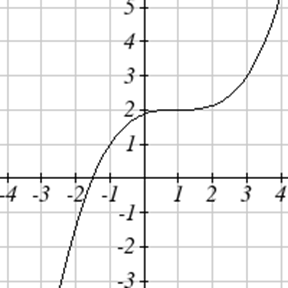
For each function graphed, estimate the intervals on which the function is increasing and decreasing.
 52.
52.