
3.2.E: Exercises
- Page ID
- 157586

\( \newcommand{\vecs}[1]{\overset { \scriptstyle \rightharpoonup} {\mathbf{#1}} } \)
\( \newcommand{\vecd}[1]{\overset{-\!-\!\rightharpoonup}{\vphantom{a}\smash {#1}}} \)
\( \newcommand{\id}{\mathrm{id}}\) \( \newcommand{\Span}{\mathrm{span}}\)
( \newcommand{\kernel}{\mathrm{null}\,}\) \( \newcommand{\range}{\mathrm{range}\,}\)
\( \newcommand{\RealPart}{\mathrm{Re}}\) \( \newcommand{\ImaginaryPart}{\mathrm{Im}}\)
\( \newcommand{\Argument}{\mathrm{Arg}}\) \( \newcommand{\norm}[1]{\| #1 \|}\)
\( \newcommand{\inner}[2]{\langle #1, #2 \rangle}\)
\( \newcommand{\Span}{\mathrm{span}}\)
\( \newcommand{\id}{\mathrm{id}}\)
\( \newcommand{\Span}{\mathrm{span}}\)
\( \newcommand{\kernel}{\mathrm{null}\,}\)
\( \newcommand{\range}{\mathrm{range}\,}\)
\( \newcommand{\RealPart}{\mathrm{Re}}\)
\( \newcommand{\ImaginaryPart}{\mathrm{Im}}\)
\( \newcommand{\Argument}{\mathrm{Arg}}\)
\( \newcommand{\norm}[1]{\| #1 \|}\)
\( \newcommand{\inner}[2]{\langle #1, #2 \rangle}\)
\( \newcommand{\Span}{\mathrm{span}}\) \( \newcommand{\AA}{\unicode[.8,0]{x212B}}\)
\( \newcommand{\vectorA}[1]{\vec{#1}} % arrow\)
\( \newcommand{\vectorAt}[1]{\vec{\text{#1}}} % arrow\)
\( \newcommand{\vectorB}[1]{\overset { \scriptstyle \rightharpoonup} {\mathbf{#1}} } \)
\( \newcommand{\vectorC}[1]{\textbf{#1}} \)
\( \newcommand{\vectorD}[1]{\overrightarrow{#1}} \)
\( \newcommand{\vectorDt}[1]{\overrightarrow{\text{#1}}} \)
\( \newcommand{\vectE}[1]{\overset{-\!-\!\rightharpoonup}{\vphantom{a}\smash{\mathbf {#1}}}} \)
\( \newcommand{\vecs}[1]{\overset { \scriptstyle \rightharpoonup} {\mathbf{#1}} } \)
\( \newcommand{\vecd}[1]{\overset{-\!-\!\rightharpoonup}{\vphantom{a}\smash {#1}}} \)
\(\newcommand{\avec}{\mathbf a}\) \(\newcommand{\bvec}{\mathbf b}\) \(\newcommand{\cvec}{\mathbf c}\) \(\newcommand{\dvec}{\mathbf d}\) \(\newcommand{\dtil}{\widetilde{\mathbf d}}\) \(\newcommand{\evec}{\mathbf e}\) \(\newcommand{\fvec}{\mathbf f}\) \(\newcommand{\nvec}{\mathbf n}\) \(\newcommand{\pvec}{\mathbf p}\) \(\newcommand{\qvec}{\mathbf q}\) \(\newcommand{\svec}{\mathbf s}\) \(\newcommand{\tvec}{\mathbf t}\) \(\newcommand{\uvec}{\mathbf u}\) \(\newcommand{\vvec}{\mathbf v}\) \(\newcommand{\wvec}{\mathbf w}\) \(\newcommand{\xvec}{\mathbf x}\) \(\newcommand{\yvec}{\mathbf y}\) \(\newcommand{\zvec}{\mathbf z}\) \(\newcommand{\rvec}{\mathbf r}\) \(\newcommand{\mvec}{\mathbf m}\) \(\newcommand{\zerovec}{\mathbf 0}\) \(\newcommand{\onevec}{\mathbf 1}\) \(\newcommand{\real}{\mathbb R}\) \(\newcommand{\twovec}[2]{\left[\begin{array}{r}#1 \\ #2 \end{array}\right]}\) \(\newcommand{\ctwovec}[2]{\left[\begin{array}{c}#1 \\ #2 \end{array}\right]}\) \(\newcommand{\threevec}[3]{\left[\begin{array}{r}#1 \\ #2 \\ #3 \end{array}\right]}\) \(\newcommand{\cthreevec}[3]{\left[\begin{array}{c}#1 \\ #2 \\ #3 \end{array}\right]}\) \(\newcommand{\fourvec}[4]{\left[\begin{array}{r}#1 \\ #2 \\ #3 \\ #4 \end{array}\right]}\) \(\newcommand{\cfourvec}[4]{\left[\begin{array}{c}#1 \\ #2 \\ #3 \\ #4 \end{array}\right]}\) \(\newcommand{\fivevec}[5]{\left[\begin{array}{r}#1 \\ #2 \\ #3 \\ #4 \\ #5 \\ \end{array}\right]}\) \(\newcommand{\cfivevec}[5]{\left[\begin{array}{c}#1 \\ #2 \\ #3 \\ #4 \\ #5 \\ \end{array}\right]}\) \(\newcommand{\mattwo}[4]{\left[\begin{array}{rr}#1 \amp #2 \\ #3 \amp #4 \\ \end{array}\right]}\) \(\newcommand{\laspan}[1]{\text{Span}\{#1\}}\) \(\newcommand{\bcal}{\cal B}\) \(\newcommand{\ccal}{\cal C}\) \(\newcommand{\scal}{\cal S}\) \(\newcommand{\wcal}{\cal W}\) \(\newcommand{\ecal}{\cal E}\) \(\newcommand{\coords}[2]{\left\{#1\right\}_{#2}}\) \(\newcommand{\gray}[1]{\color{gray}{#1}}\) \(\newcommand{\lgray}[1]{\color{lightgray}{#1}}\) \(\newcommand{\rank}{\operatorname{rank}}\) \(\newcommand{\row}{\text{Row}}\) \(\newcommand{\col}{\text{Col}}\) \(\renewcommand{\row}{\text{Row}}\) \(\newcommand{\nul}{\text{Nul}}\) \(\newcommand{\var}{\text{Var}}\) \(\newcommand{\corr}{\text{corr}}\) \(\newcommand{\len}[1]{\left|#1\right|}\) \(\newcommand{\bbar}{\overline{\bvec}}\) \(\newcommand{\bhat}{\widehat{\bvec}}\) \(\newcommand{\bperp}{\bvec^\perp}\) \(\newcommand{\xhat}{\widehat{\xvec}}\) \(\newcommand{\vhat}{\widehat{\vvec}}\) \(\newcommand{\uhat}{\widehat{\uvec}}\) \(\newcommand{\what}{\widehat{\wvec}}\) \(\newcommand{\Sighat}{\widehat{\Sigma}}\) \(\newcommand{\lt}{<}\) \(\newcommand{\gt}{>}\) \(\newcommand{\amp}{&}\) \(\definecolor{fillinmathshade}{gray}{0.9}\)3.2 Exercises
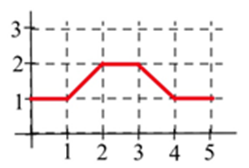
Let \(A(x)\) represent the area bounded by the graph and the horizontal axis and vertical lines at \(t=0\) and \(t=x\) for the graph shown. Evaluate \(A(x)\) for \(x =\) 1, 2, 3, 4, and 5.
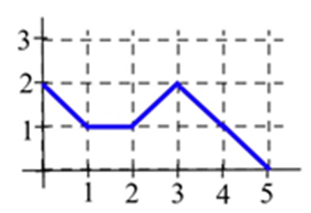
Let \(B(x)\) represent the area bounded by the graph and the horizontal axis and vertical lines at \(t=0\) and \(t=x\) for the graph shown. Evaluate \(B(x)\) for \(x =\) 1, 2, 3, 4, and 5.
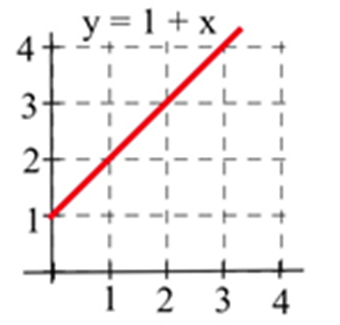
Let \(C(x)\) represent the area bounded by the graph and the horizontal axis and vertical lines at \(t=0\) and \(t=x\) for the graph shown. Evaluate \(C(x)\) for \(x =\) 1, 2, and 3 and find a formula for \(C(x)\).
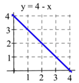
Let \(A(x)\) represent the area bounded by the graph and the horizontal axis and vertical lines at \(t=0\) and \(t=x\) for the graph shown. Evaluate \(A(x)\) for \(x =\) 1, 2, and 3 and find a formula for \(A(x)\).
A car had the velocity shown in the graph to the right.
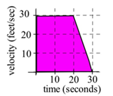
A car had the velocity shown in the graph to the right. How far did the car travel from \(t= 0\) to \(t = 30\) seconds?
A car had the velocity shown below.
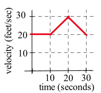
How afar did the car travel from \(t = 0\) to \(t = 30\) seconds?
The velocities of two cars are shown in the graph.
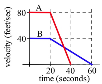
(a) From the time the brakes were applied, how many seconds did it take each car to stop?
(b) From the time the brakes were applied, which car traveled farther until it came to a complete stop?
You and a friend start off at noon and walk in the same direction along the same path at the rates shown.
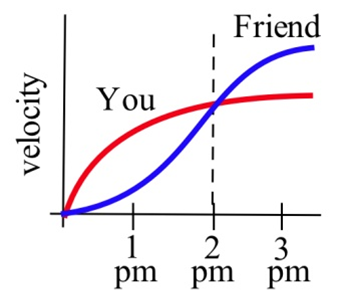
(a) Who is walking faster at 2 pm? Who is ahead at 2 pm?
(b) Who is walking faster at 3 pm? Who is ahead at 3 pm?
(c) When will you and your friend be together? (Answer in words.)
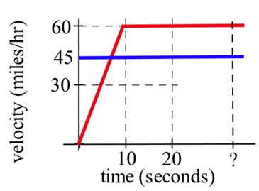
Police chase: A speeder traveling 45 miles per hour (in a 25 mph zone) passes a stopped police car which immediately takes off after the speeder. If the police car speeds up steadily to 60 miles/hour in 20 seconds and then travels at a steady 60 miles/hour, how long and how far before the police car catches the speeder who continued traveling at 45 miles/hour?
Water is flowing into a tub. The table shows the rate at which the water flows, in gallons per minute. The tub is initially empty.
|
\(t\), in minutes |
0 |
1 |
2 |
3 |
4 |
5 |
6 |
7 |
8 |
9 |
10 |
|
Flow rate, in gal/min |
0.5 |
1.0 |
1.2 |
1.4 |
1.7 |
2.0 |
2.3 |
1.8 |
0.7 |
0.5 |
0.2 |
Use the table to estimate how much water is in the tub after
a. five minutes
b. ten minutes
The table shows the speedometer readings for a short car trip.
|
\(t\), in minutes |
0 |
5 |
10 |
15 |
20 |
|
Speed, in mph |
0 |
30 |
40 |
65 |
40 |
a. Use the table to estimate how far the car traveled over the twenty minutes shown.
b. How accurate would you expect your estimate to be?
The table shows values of \(f(t)\). Use the table to estimate \(\int^{40}_0 f(t) dt\).
|
\(t\) |
0 |
10 |
20 |
30 |
40 |
|
\(f(t)\) |
17 |
22 |
18 |
11 |
35 |
The table shows values of \(g(x)\).
|
\(x\) |
0 |
1 |
2 |
3 |
4 |
5 |
6 |
|
\(g(x)\) |
140 |
142 |
144 |
152 |
154 |
165 |
200 |
Use the table to estimate
| a. \(\int^3_0 g(x) dx\) | b \(\int^6_3 g(x) dx\) | c. \(\int^6_0 g(x) dx\) |
What are the units for the "area" of a rectangle with the given base and height units?
| Base units | Height units | "Area" units |
|
miles per second |
seconds |
|
|
hours |
dollars per hour |
|
|
square feet |
feet |
|
|
kilowatts |
hours |
|
|
houses |
people per house |
|
|
meals |
meals |
In problems 15 – 17, represent the area of each bounded region as a definite integral, and use geometry to determine the value of the definite integral.
15. The region bounded by \(y = 2x \), the \(x\)–axis, the line \(x = 1\), and \(x = 3\).
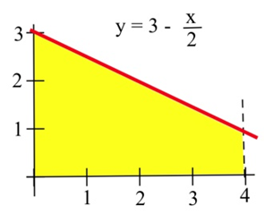
16. The region bounded by \(y = 4 – 2x \), the \(x\)–axis, and the \(y\)–axis.
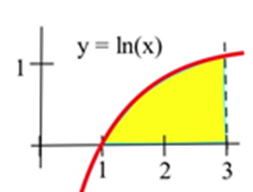
17. The shaded region in the graph to the right.
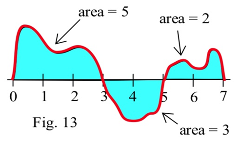
Using the graph of \(f\) shown and the given areas of several regions, evaluate:
(a) \(\int^3_0 f(x) dx\)
(b) \(\int^5_3 f(x) dx\)
(c) \(\int^7_5 f(x) dx\)
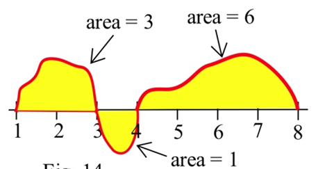
Using the graph of \(f\) shown and the given areas of several regions, evaluate:
(a) \(\int^3_1 g(x) dx\)
(b) \(\int^4_3 g(x) dx\)
(c) \(\int^8_4 g(x) dx\)
(d) \(\int^8_1 g(x) dx\)
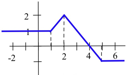
Use the graph to evaluate:
(a) \(\int^1_{-2} h(x) dx\)
(b) \(\int^6_4 h(x) dx\)
(c) \(\int^6_{-2} h(x) dx\)
(d) \(\int^4_{-2} h(x) dx\)
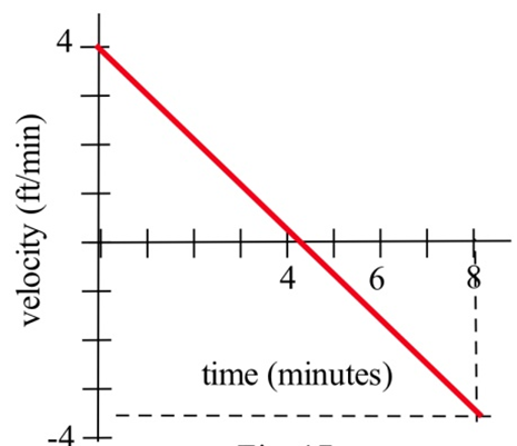
Your velocity along a straight road is shown to the right. How far did you travel in 8 minutes?
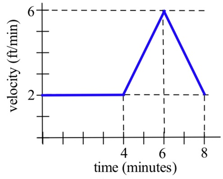
Your velocity along a straight road is shown below. How many feet did you walk in 8 minutes?
In problems 23 - 26, the units are given for \(x\) and for \(f(x)\). Give the units of \(\int^b_a f(x) dx\).
23. \(x\) is time in "seconds", and \(f(x)\) is velocity in "meters per second."
24. \(x\) is time in "hours", and \(f(x)\) is a flow rate in "gallons per hour."
25. \(x\) is a position in "feet", and \(f(x)\) is an area in "square feet."
26. \(x\) is a position in "inches", and \(f(x)\) is a density in "pounds per inch."
In problems 27 – 31, represent the area with a definite integral and use technology to find the approximate answer.
27. The region bounded by \(y = x^3\), the \(x\)–axis, the line \(x = 1\), and \(x = 5\).
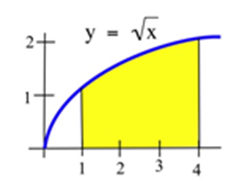
28. The region bounded by \(y = \sqrt{x}\), the \(x\)–axis, and the line \(x = 9\).
29. The shaded region shown to the right.
30. The shaded region below.
31. Consider the definite integral \(\int^3_0 (3+x) dx\).
(a) Using six rectangles, find the left-hand Riemann sum for this definite integral.
(b) Using six rectangles, find the right-hand Riemann sum for this definite integral.
(c) Using geometry, find the exact value of this definite integral.
Consider the definite integral \(\int^2_0 x^3 dx\).
(a) Using four rectangles, find the left-hand Riemann sum for this definite integral.
(b) Using four rectangles, find the right-hand Riemann sum for this definite integral.
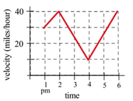
Write the total distance traveled by the car in the graph between 1 pm and 4 pm as a definite integral and estimate the value of the integral.
Problems 34 – 41 refer to the graph of \(f\) shown.
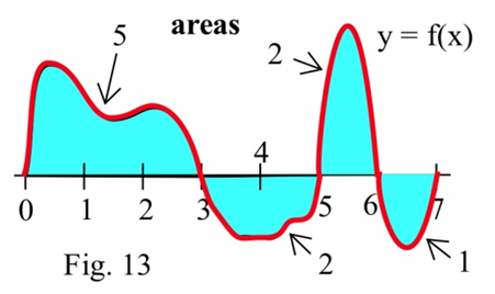
Use the graph to determine the values of the definite integrals. (The bold numbers represent the area of each region.)
| 34. \(\int^3_0 f(x) dx\) | 35. \(\int^5_3 f(x) dx\) | 36. \(\int^2_2 f(x) dx\) | 37. \(\int^7_6 f(w) dw\) |
| 38. \(\int^5_0 f(x) dx\) | 39. \(\int^7_0 f(x) dx\) | 40. \(\int^6_3 f(t) dt\) | 41. \(\int^7_5 f(x) dx\) |
Problems 42 – 47 refer to the graph of \(g\) shown.
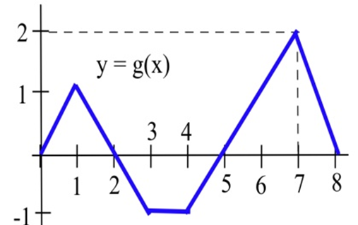
Use the graph to evaluate the integrals.
| 42. \(\int^2_0 g(x) dx\) | 43. \(\int^3_1 g(t) dt\) | 44. \(\int^5_0 g(x) dx\) |
| 45. \(\int^8_0 g(s) ds\) | 46. \(\int^3_0 2g(t) dt\) | 47. \(\int^8_5 1+g(x) dx\) |