

3.7.E: Exercises
- Page ID
- 157591

\( \newcommand{\vecs}[1]{\overset { \scriptstyle \rightharpoonup} {\mathbf{#1}} } \)
\( \newcommand{\vecd}[1]{\overset{-\!-\!\rightharpoonup}{\vphantom{a}\smash {#1}}} \)
\( \newcommand{\dsum}{\displaystyle\sum\limits} \)
\( \newcommand{\dint}{\displaystyle\int\limits} \)
\( \newcommand{\dlim}{\displaystyle\lim\limits} \)
\( \newcommand{\id}{\mathrm{id}}\) \( \newcommand{\Span}{\mathrm{span}}\)
( \newcommand{\kernel}{\mathrm{null}\,}\) \( \newcommand{\range}{\mathrm{range}\,}\)
\( \newcommand{\RealPart}{\mathrm{Re}}\) \( \newcommand{\ImaginaryPart}{\mathrm{Im}}\)
\( \newcommand{\Argument}{\mathrm{Arg}}\) \( \newcommand{\norm}[1]{\| #1 \|}\)
\( \newcommand{\inner}[2]{\langle #1, #2 \rangle}\)
\( \newcommand{\Span}{\mathrm{span}}\)
\( \newcommand{\id}{\mathrm{id}}\)
\( \newcommand{\Span}{\mathrm{span}}\)
\( \newcommand{\kernel}{\mathrm{null}\,}\)
\( \newcommand{\range}{\mathrm{range}\,}\)
\( \newcommand{\RealPart}{\mathrm{Re}}\)
\( \newcommand{\ImaginaryPart}{\mathrm{Im}}\)
\( \newcommand{\Argument}{\mathrm{Arg}}\)
\( \newcommand{\norm}[1]{\| #1 \|}\)
\( \newcommand{\inner}[2]{\langle #1, #2 \rangle}\)
\( \newcommand{\Span}{\mathrm{span}}\) \( \newcommand{\AA}{\unicode[.8,0]{x212B}}\)
\( \newcommand{\vectorA}[1]{\vec{#1}} % arrow\)
\( \newcommand{\vectorAt}[1]{\vec{\text{#1}}} % arrow\)
\( \newcommand{\vectorB}[1]{\overset { \scriptstyle \rightharpoonup} {\mathbf{#1}} } \)
\( \newcommand{\vectorC}[1]{\textbf{#1}} \)
\( \newcommand{\vectorD}[1]{\overrightarrow{#1}} \)
\( \newcommand{\vectorDt}[1]{\overrightarrow{\text{#1}}} \)
\( \newcommand{\vectE}[1]{\overset{-\!-\!\rightharpoonup}{\vphantom{a}\smash{\mathbf {#1}}}} \)
\( \newcommand{\vecs}[1]{\overset { \scriptstyle \rightharpoonup} {\mathbf{#1}} } \)
\(\newcommand{\longvect}{\overrightarrow}\)
\( \newcommand{\vecd}[1]{\overset{-\!-\!\rightharpoonup}{\vphantom{a}\smash {#1}}} \)
\(\newcommand{\ket}[1]{\left| #1 \right>}\)
\(\newcommand{\bra}[1]{\left< #1 \right|}\)
\(\newcommand{\braket}[2]{\left< #1 \vphantom{#2} \right| \left. #2 \vphantom{#1} \right>}\)
\(\newcommand{\braopket}[3]{\left< #1 \vphantom{#2}\vphantom{#3} \right| #2 \vphantom{#1}\vphantom{#3} \left| #3 \vphantom{#1}\vphantom{#2} \right>}\)
\(\newcommand{\qmvec}[1]{\mathbf{\vec{#1}}}\)
\(\newcommand{\op}[1]{\hat{\mathbf{#1}}}\)
\(\newcommand{\expect}[1]{\langle #1 \rangle}\)
\(\newcommand{\dfn}[1]{\emph{\textbf{#1}}}\)
3.7 Exercises
In problems 1 – 4, use the values in the table to estimate the areas.
| \(x\) | \(f(x)\) | \(g(x)\) | \(h(x)\) |
|
0 |
5 |
2 |
5 |
|
1 |
6 |
1 |
6 |
|
2 |
6 |
2 |
8 |
|
3 |
4 |
2 |
6 |
|
4 |
3 |
3 |
5 |
|
5 |
2 |
4 |
4 |
|
6 |
2 |
0 |
2 |
1. Estimate the area between \(f\) and \(g\), between \(x = 0\) and \(x = 4\).
2. Estimate the area between \(g\) and \(h\), between \(x = 0\) and \(x = 6\).
3. Estimate the area between \(f\) and \(h\), between \(x = 0\) and \(x = 4\).
4. Estimate the area between \(f\) and \(g\), between \(x = 0\) and \(x = 6\).
Estimate the area of the island shown
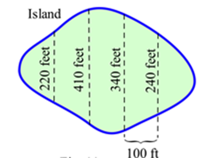
In problems 6 – 15, find the area between the graphs of \(f\) and \(g\) for \(x\) in the given interval. Remember to draw the graph!
| 6. \(f(x) = x^2 + 3 \), \(g(x) = 1\) and \(–1 \leq x \leq 2\). |
| 7. \(f(x) = x^2 + 3 \), \(g(x) = 1 + x\) and \(0 \leq x \leq 3\). |
| 8. \(f(x) = x^2 \), \(g(x) = x\) and \(0 \leq x \leq 2\). |
| 9. \(f(x) = (x –1)^2 \), \(g(x) = x + 1\) and \(0 \leq x \leq 3\). |
| 10. \(f(x) = \frac{1}{x}\), \(g(x) = x\) and \(1 \leq x \leq e\). |
| 11. \(f(x) = \sqrt{x}\), \(g(x) = x\) and \(0 \leq x \leq 4\). |
| 12. \(f(x) = 4 – x^2 \), \(g(x) = x + 2\) and \(0 \leq x \leq 2\). |
| 13. \(f(x) = e^x\), \(g(x) = x\) and \(0 \leq x \leq 2\). |
| 14. \(f(x) = 3 \), \(g(x) = \sqrt{1-x^2}\) and \(0 \leq x \leq 1\). |
| 15. \(f(x) = 2 \), \(g(x) = \sqrt{4-x^2}\) and \(–2 \leq x \leq 2\). |
For problems 16-18, find the volume of the solid obtained by rotating the specified region about the \(x\) axis.
16. Region under \(f(x) = x^2 + 3\) for \(–1 \leq x \leq 2\).
17. Region under \(f(x) = 4 – x^2\) for \(0 \leq x \leq 2\).
18. Region under \(f(x) = \frac{1}{x}\) for \(1 \leq x \leq 2\).
In problems 19 and 20 use the values in the table to estimate the average values.
| \(x\) | \(f(x)\) | \(g(x)\) |
|
0 |
5 |
2 |
|
1 |
6 |
1 |
|
2 |
6 |
2 |
|
3 |
4 |
2 |
|
4 |
3 |
3 |
|
5 |
2 |
4 |
|
6 |
2 |
0 |
19. Estimate the average value of \(f\) on the interval [0, 6].
20. Estimate the average value of \(g\) on the interval [0, 6].
In problems 21 – 26, find the average value of \(f\) on the given interval.
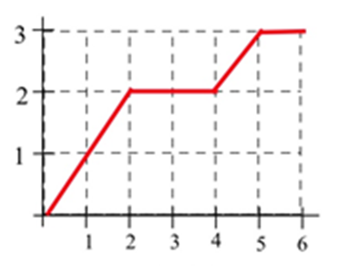
21. \(f(x)\) from the graph for \(0 \leq x \leq 2\).
22. \(f(x)\) from the graph for \(0 \leq x \leq 4\).
23. \(f(x)\) from the graph for \(1 \leq x \leq 6\).
24. \(f(x)\) from the graph for \(4 \leq x \leq 6\).
25. \(f(x) = 2x + 1\) for \(0 \leq x \leq 4\).
26. \(f(x) = x^2\) for \(0 \leq x \leq 2\).
The graph shows the velocity of a car during a 5 hour trip.
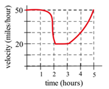
(a) Estimate how far the car traveled during the 5 hours.
(b) At what constant velocity should you drive in order to travel the same distance in 5 hours?
The graph shows the number of telephone calls per minute at a large company.
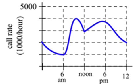
Estimate the average number of calls per minute
(a) From 8 am to 5 pm.
(b) From 9 am to 1 pm.