
4.1.E: Exercises
- Page ID
- 157594

\( \newcommand{\vecs}[1]{\overset { \scriptstyle \rightharpoonup} {\mathbf{#1}} } \)
\( \newcommand{\vecd}[1]{\overset{-\!-\!\rightharpoonup}{\vphantom{a}\smash {#1}}} \)
\( \newcommand{\id}{\mathrm{id}}\) \( \newcommand{\Span}{\mathrm{span}}\)
( \newcommand{\kernel}{\mathrm{null}\,}\) \( \newcommand{\range}{\mathrm{range}\,}\)
\( \newcommand{\RealPart}{\mathrm{Re}}\) \( \newcommand{\ImaginaryPart}{\mathrm{Im}}\)
\( \newcommand{\Argument}{\mathrm{Arg}}\) \( \newcommand{\norm}[1]{\| #1 \|}\)
\( \newcommand{\inner}[2]{\langle #1, #2 \rangle}\)
\( \newcommand{\Span}{\mathrm{span}}\)
\( \newcommand{\id}{\mathrm{id}}\)
\( \newcommand{\Span}{\mathrm{span}}\)
\( \newcommand{\kernel}{\mathrm{null}\,}\)
\( \newcommand{\range}{\mathrm{range}\,}\)
\( \newcommand{\RealPart}{\mathrm{Re}}\)
\( \newcommand{\ImaginaryPart}{\mathrm{Im}}\)
\( \newcommand{\Argument}{\mathrm{Arg}}\)
\( \newcommand{\norm}[1]{\| #1 \|}\)
\( \newcommand{\inner}[2]{\langle #1, #2 \rangle}\)
\( \newcommand{\Span}{\mathrm{span}}\) \( \newcommand{\AA}{\unicode[.8,0]{x212B}}\)
\( \newcommand{\vectorA}[1]{\vec{#1}} % arrow\)
\( \newcommand{\vectorAt}[1]{\vec{\text{#1}}} % arrow\)
\( \newcommand{\vectorB}[1]{\overset { \scriptstyle \rightharpoonup} {\mathbf{#1}} } \)
\( \newcommand{\vectorC}[1]{\textbf{#1}} \)
\( \newcommand{\vectorD}[1]{\overrightarrow{#1}} \)
\( \newcommand{\vectorDt}[1]{\overrightarrow{\text{#1}}} \)
\( \newcommand{\vectE}[1]{\overset{-\!-\!\rightharpoonup}{\vphantom{a}\smash{\mathbf {#1}}}} \)
\( \newcommand{\vecs}[1]{\overset { \scriptstyle \rightharpoonup} {\mathbf{#1}} } \)
\( \newcommand{\vecd}[1]{\overset{-\!-\!\rightharpoonup}{\vphantom{a}\smash {#1}}} \)
\(\newcommand{\avec}{\mathbf a}\) \(\newcommand{\bvec}{\mathbf b}\) \(\newcommand{\cvec}{\mathbf c}\) \(\newcommand{\dvec}{\mathbf d}\) \(\newcommand{\dtil}{\widetilde{\mathbf d}}\) \(\newcommand{\evec}{\mathbf e}\) \(\newcommand{\fvec}{\mathbf f}\) \(\newcommand{\nvec}{\mathbf n}\) \(\newcommand{\pvec}{\mathbf p}\) \(\newcommand{\qvec}{\mathbf q}\) \(\newcommand{\svec}{\mathbf s}\) \(\newcommand{\tvec}{\mathbf t}\) \(\newcommand{\uvec}{\mathbf u}\) \(\newcommand{\vvec}{\mathbf v}\) \(\newcommand{\wvec}{\mathbf w}\) \(\newcommand{\xvec}{\mathbf x}\) \(\newcommand{\yvec}{\mathbf y}\) \(\newcommand{\zvec}{\mathbf z}\) \(\newcommand{\rvec}{\mathbf r}\) \(\newcommand{\mvec}{\mathbf m}\) \(\newcommand{\zerovec}{\mathbf 0}\) \(\newcommand{\onevec}{\mathbf 1}\) \(\newcommand{\real}{\mathbb R}\) \(\newcommand{\twovec}[2]{\left[\begin{array}{r}#1 \\ #2 \end{array}\right]}\) \(\newcommand{\ctwovec}[2]{\left[\begin{array}{c}#1 \\ #2 \end{array}\right]}\) \(\newcommand{\threevec}[3]{\left[\begin{array}{r}#1 \\ #2 \\ #3 \end{array}\right]}\) \(\newcommand{\cthreevec}[3]{\left[\begin{array}{c}#1 \\ #2 \\ #3 \end{array}\right]}\) \(\newcommand{\fourvec}[4]{\left[\begin{array}{r}#1 \\ #2 \\ #3 \\ #4 \end{array}\right]}\) \(\newcommand{\cfourvec}[4]{\left[\begin{array}{c}#1 \\ #2 \\ #3 \\ #4 \end{array}\right]}\) \(\newcommand{\fivevec}[5]{\left[\begin{array}{r}#1 \\ #2 \\ #3 \\ #4 \\ #5 \\ \end{array}\right]}\) \(\newcommand{\cfivevec}[5]{\left[\begin{array}{c}#1 \\ #2 \\ #3 \\ #4 \\ #5 \\ \end{array}\right]}\) \(\newcommand{\mattwo}[4]{\left[\begin{array}{rr}#1 \amp #2 \\ #3 \amp #4 \\ \end{array}\right]}\) \(\newcommand{\laspan}[1]{\text{Span}\{#1\}}\) \(\newcommand{\bcal}{\cal B}\) \(\newcommand{\ccal}{\cal C}\) \(\newcommand{\scal}{\cal S}\) \(\newcommand{\wcal}{\cal W}\) \(\newcommand{\ecal}{\cal E}\) \(\newcommand{\coords}[2]{\left\{#1\right\}_{#2}}\) \(\newcommand{\gray}[1]{\color{gray}{#1}}\) \(\newcommand{\lgray}[1]{\color{lightgray}{#1}}\) \(\newcommand{\rank}{\operatorname{rank}}\) \(\newcommand{\row}{\text{Row}}\) \(\newcommand{\col}{\text{Col}}\) \(\renewcommand{\row}{\text{Row}}\) \(\newcommand{\nul}{\text{Nul}}\) \(\newcommand{\var}{\text{Var}}\) \(\newcommand{\corr}{\text{corr}}\) \(\newcommand{\len}[1]{\left|#1\right|}\) \(\newcommand{\bbar}{\overline{\bvec}}\) \(\newcommand{\bhat}{\widehat{\bvec}}\) \(\newcommand{\bperp}{\bvec^\perp}\) \(\newcommand{\xhat}{\widehat{\xvec}}\) \(\newcommand{\vhat}{\widehat{\vvec}}\) \(\newcommand{\uhat}{\widehat{\uvec}}\) \(\newcommand{\what}{\widehat{\wvec}}\) \(\newcommand{\Sighat}{\widehat{\Sigma}}\) \(\newcommand{\lt}{<}\) \(\newcommand{\gt}{>}\) \(\newcommand{\amp}{&}\) \(\definecolor{fillinmathshade}{gray}{0.9}\)4.1 Exercises
\(F(x,y) = x^2-y^2\). Find
a) \(F(0,4)\)
b) \(F(4,0)\)
c) \(F(x,4)\)
d) \(F(4,y)\)
e) \(F(800,800)\)
f) \(F(x,x)\)
g) \(F(x,-x)\)
\(g(s,t)=\sqrt{st^2}\). Find
a) \(g(1,9)\)
b) \(g(9,1)\)
c) \(g(1,t)\)
d) \(g(s,9)\)
e) \(g(w,z+1)\)
Let \(f(x,y,z,w) = x^2 - \frac{1}{zw}+xyz^2\). Evaluate \(f(1,2,3,4)\).
Let \(f(x,y,z,w) = \sqrt{xy} - w^2 + 102yz\). Evaluate \(f(1,2,3,4)\).
Here is a table showing the function \(A(t,r)\)
| \(\overset{t}{\downarrow} \ r\rightarrow\) |
.03 |
.04 |
.05 |
.06 |
.07 |
|
1 |
30.45 |
40.81 |
51.27 |
61.84 |
72.51 |
|
2 |
61.84 |
83.29 |
105.17 |
127.50 |
150.27 |
|
3 |
94.17 |
127.50 |
161.83 |
197.22 |
233.68 |
a) Find \(A(2, .05)\)
b) Find \(A(.05, .2)\)
c) Is \(A(t, .06)\) an increasing or decreasing function of \(t \)?
d) Is \(A(3, r)\) an increasing or decreasing function of \(r\)?
Here is a table showing values for the function \(H(t,h)\).
| \(\overset{t}{\downarrow} \ h\rightarrow\) |
100 |
150 |
200 |
|
0 |
100 |
150 |
200 |
|
1 |
110.1 |
160.1 |
210.1 |
|
2 |
110.4 |
160.4 |
210.4 |
|
3 |
100.9 |
150.9 |
200.9 |
|
4 |
81.6 |
131.6 |
181.6 |
|
5 |
52.5 |
102.5 |
152.5 |
a) Is \(H(t, 150)\) an increasing or decreasing function of \(t \)?
b) Is \(H( 4, h)\) an increasing or decreasing function of \(h\)?
c) Fill in the blanks: The maximum value shown on this table is \(H\)(___,___) =____.
d) Fill in the blanks: The minimum value shown on this table is \(H\)(___,___) =____.
In problems 7 – 10, plot the given points.
7. \(A = (0,3,4), B = (1,4,0), C = (1,3,4), D = (1, 4,2)\)
8. \(E = (4,3,0), F = (3,0,1), G = (0,4,1), H = (3,3,1)\)
9. \(P = (2,3,–4), Q = (1,–2,3), R = (4,–1,–2), S = (–2,1,3)\)
10. \(T = (–2,3,–4), U = (2,0,–3), V = (–2,0,0), W = (–3,–1,–2)\)
In problems 11 – 14, calculate the distances between the given points
11. \(A = (5,3,4), B = (3,4,4)\)
12. \(A = (6,2,1), B = (3,2,1)\)
13. \(A = (3,4,2), B = (–1,6,–2)\)
14. \(A = (–1,5,0), B = (1,3,2)\)
In problems 15 – 18, graph the given planes.
| 15. \(y = 1\) and \(z = 2\) | 16. \(x = 4\) and \(y = 2\) |
| 17. \(x = 1\) and \(y = 0\) | 18. \(x = 2\) and \(z = 0\) |
In problems 19 – 22, the center and radius of a sphere are given. Find an equation for the sphere.
| 19. Center = (4, 3, 5), radius = 3 | 20. Center = (0, 3, 6), radius = 2 |
| 21. Center = (5, 1, 0), radius = 5 | 22. Center = (1, 2, 3), radius = 4 |
In problems 23 – 24, the equation of a sphere is given. Find the center and radius of the sphere.
| 23. \((x–3)^2 + (y+4)^2 + (z–1)^2 = 16\) | 24. \((x+2)^2 + y^2 + (z–4)^2 = 25\) |
For problems 25 through 30. Match the contour diagram to the computer-generated, perspective drawing (a through f) it matches. Briefly explain your answer.
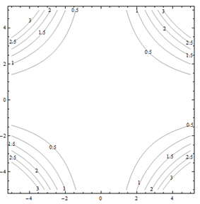

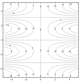
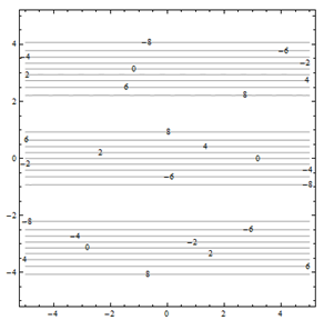

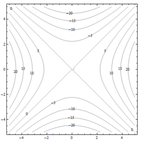
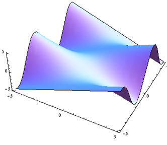
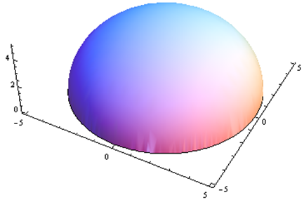
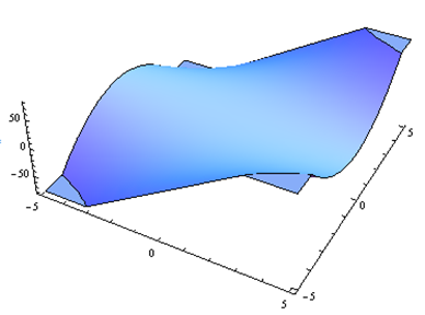
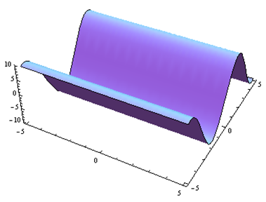
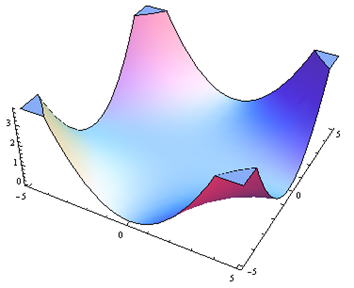
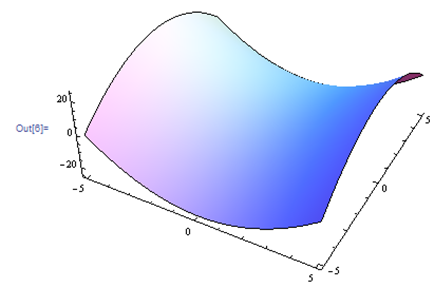
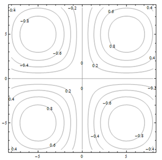
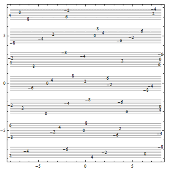
For problems 31 through 36. Match the contour diagram to the equation (a through f) it matches. Briefly explain your answer.

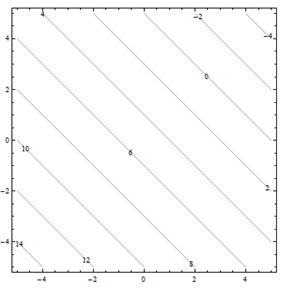
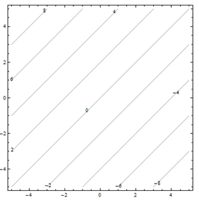

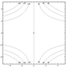
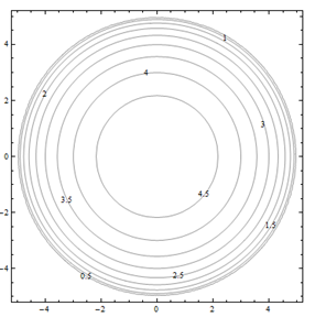
| a. \(f(x,y) = y-x\) | b. \(f(x,y) = xy^2\) |
| c. \(f(x,y) = \sqrt{25-x^2-y^2}\) | d. \(f(x,y) = 5-x-y\) |
| e. \(f(x,y) = 0.01x^2y^2\) | f. \(f(x,y) = x^2-y^2\) |
The contour diagram shown is for a function \(M(x, y)\).
Use the diagram to answer the following:
a) Estimate \(M(1, 3)\)
b) Estimate \(M(3, 1)\)
c) Is \(M(x, 3)\) an increasing or decreasing function of \(x\)?
d) Is \(M(3, y)\) an increasing or decreasing function of \(y\)?
e) Find a value of \(c\) so that \(M(c, y)\) is a constant function of \(y\).
The contour diagram shown is for a function \(G(x, y)\).
Use the diagram to answer the following:
a) Estimate \(G(2, 3)\)
b) Suppose you travel north (in the direction of increasing \(y\)) along the surface, starting above (2, 3). Describe your journey.
c) Suppose you travel east (in the direction of increasing \(x\)) along the surface, starting above (2, 3). Describe your journey.
The demand functions for two products are given below. \(p_1\), \(p_2\), \(q_1\), and \(q_2\) are the prices (in dollars) and quantities for products 1 and 2. Are these two products complementary goods or substitute goods
\[q_1 = 200 -3p_1 + p_2 \nonumber\]
\[q_2 = 150 + p_1 -2p_2 \nonumber\]
The demand functions for two products are given below. \(p_1\), \(p_2\), \(q_1\), and \(q_2\) are the prices (in dollars) and quantities for products 1 and 2. Are these two products complementary goods or substitute goods
\[q_1 = 350 + p_1 + 2p_2 \nonumber\]
\[q_2 = 225 + p_1 + p_2 \nonumber\]
Consider the Cobb-Douglas Production function: \(P(L,K) = 11 L^{0.3} K^{0.7}\). Find the total units of production when 19 units of labor and 12 units of capital are invested.
Consider the Cobb-Douglas Production function: \(P(L,K) = 6 L^{0.6} K^{0.4}\). Find the total units of production when 24 units of labor and 8 units of capital are invested.