In other words, a parallelepiped is the set of all linear combinations of \(n\) vectors with coefficients in \([0,1]\). We can draw parallelepipeds using the parallelogram law for vector addition.
Example \(\PageIndex{1}\): The Unit Cube
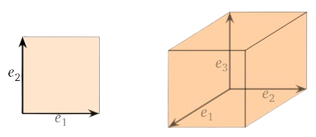
The parallelepiped determined by the standard coordinate vectors \(\vec{e}_1,\vec{e}_2,\ldots,\vec{e}_n\) is the unit \(n\)-dimensional cube.
Figure \(\PageIndex{1}\): A 2D square with axes \( \vec{e}_1 \) and \( \vec{e}_2 \) on the left, and a 3D cube with axes \( \vec{e}_1 \), \( \vec{e}_2 \), and \( \vec{e}_3 \) on the right, representing coordinate systems. (CC-BY-SA; Margalit and Rabinoff via Interactive Linear Algebra)
Example \(\PageIndex{2}\): Parallelograms
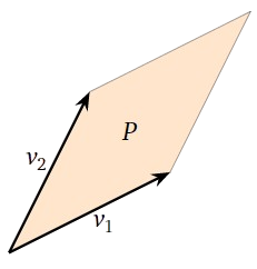
When \(n = 2\text{,}\) a parallelepiped is just a parallelogram in \(\mathbb{R}^2 \). Note that the edges come in parallel pairs.
Figure \(\PageIndex{2}\): A parallelogram \( P \) formed by vectors \( \vec{v}_1 \) and \( \vec{v}_2 \), represented as black arrows from a common point. (CC-BY-SA; Margalit and Rabinoff via Interactive Linear Algebra)
Example \(\PageIndex{3}\)
When \(n=3\text{,}\) a parallelepiped is a kind of a skewed cube. Note that the faces come in parallel pairs.
Figure \(\PageIndex{3}\): A parallelepiped \( P \) formed by vectors \( \vec{v}_1 \), \( \vec{v}_2 \), and \( \vec{v}_3 \), represented as black arrows from a common point. (CC-BY-SA; Margalit and Rabinoff via Interactive Linear Algebra)
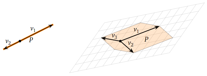
When does a parallelepiped have zero volume? This can happen only if the parallelepiped is flat, i.e., it is squashed into a lower dimension.
Figure \(\PageIndex{4}\): An illustration comparing geometric objects in one and two dimensions. On the left, a one-dimensional space is represented by a line segment with two vectors, \( \vec{v}_1 \) and \( \vec{v}_2 \), extending in opposite directions from a point \( P \). On the right, a two-dimensional parallelogram is shown lying in a tilted plane on a grid. The parallelogram is defined by three vectors, \( \vec{v}_1, \vec{v}_2, \) and \( \vec{v}_3 \), originating from a common point \( P \) and forming a shaded area. (CC-BY-SA; Margalit and Rabinoff via Interactive Linear Algebra)
This means exactly that the set \(\{\vec{v}_1,\vec{v}_2,\ldots,\vec{v}_n\}\) has some dependence, implying that the matrix with rows \(\vec{v}_1,\vec{v}_2,\ldots,\vec{v}_n\) has determinant zero. To summarize:
Key Observation \(\PageIndex{1}\)
The parallelepiped defined by \(\vec{v}_1,\vec{v}_2,\ldots,\vec{v}_n\) has zero volume if and only if the matrix with rows \(\vec{v}_1,\vec{v}_2,\ldots,\vec{v}_n\) has zero determinant.
Determinants and Volumes
The key observation above is only the beginning of the story: the volume of a parallelepiped is always a determinant.
Theorem \(\PageIndex{1}\):Determinants and Volumes
Let \(\vec{v}_1,\vec{v}_2,\ldots,\vec{v}_n\) be vectors in \(\mathbb{R}^n \text{,}\) let \(P\) be the parallelepiped determined by these vectors, and let \(A\) be the matrix with rows \(\vec{v}_1,\vec{v}_2,\ldots,\vec{v}_n\). Then the absolute value of the determinant of \(A\) is the volume of \(P\text{:}\)
\[ |\det(A)| = \text{vol}(P). \nonumber \]
Proof
Case 1: There is a dependence in the vectors \(\vec{v}_1,\vec{v}_2,\ldots,\vec{v}_n\). In this case, we established that the volume of the parallelopiped is \(0\) in Key Observation \(\PageIndex{1}\).
Case 2: There is no dependence in the vectors \(\vec{v}_1,\vec{v}_2,\ldots,\vec{v}_n\). Hence the matrix \(A\) must row reduce to \(I_n\). Suppose the required row operations correspond to left multiplying the row of \(A\) by elementary matrices \(E_1, E_2, \ldots, E_k\). That is
\[ E_m \ldots E_2 E_1 A = I_n \nonumber \]
Since all elementary matrices are invertible and are elementary matrices themselves, we can express the above relationship as
\[ A = E^{-1}_1 E^{-1}_2 \ldots E^{-1}_m I_n \nonumber \]
Let's begin with the \(n \times n\) identity matrix \(I_n\). This matrix consists of row vectors \(\vec{e}_1, \vec{e}_2, \ldots, \vec{e}_n\). The volume of the parallelepiped formed by these vectors is \(1\).
Now let us apply the opposite of the elementary row operations in reverse used to row reduce \(A\) to \(I_n\). This would give us the row operations needed to transform \(I_n\) to \(A\) using elementary row operations. What effect do these row operations have on the absolute value of the determinant?
We begin with \(I_n\), and note that \( |\det(I_n)| = 1\).
Suppose the next row operation consists of switching two rows. Switching two rows of a matrix just reorders the vectors \(v_1,v_2,\ldots,v_n\text{,}\) hence has no effect on the parallelepiped determined by those vectors. Thus, the volume is unchanged by row swaps. The determinant after swapping rows will be negative, but the absolute value of the determinant is unchanged.
Figure \(\PageIndex{5}\): A diagram illustrating the effect of row swapping on area and volume in linear algebra. In the top row, two parallelograms are shown. On the left, the parallelogram is defined by vectors \( \vec{v}_1 \) and \( \vec{v}_2 \), with \( \vec{v}_1 \) positioned as the first vector and \( \vec{v}_2 \) as the second. On the right, the parallelogram remains the same in shape and size, but the roles of \( \vec{v}_1 \) and \( \vec{v}_2 \) are swapped. This transformation demonstrates that swapping two rows negates the determinant. In the bottom row, two parallelepipeds are shown. On the left, the parallelepiped is defined by vectors \( \vec{v}_1, \vec{v}_2, \) and \( \vec{v}_3 \), with the volume determined by their orientation. On the right, \( \vec{v}_2 \) and \( \vec{v}_3 \) have swapped places, maintaining the shape but flipping the determinant’s sign. (CC-BY-SA; Margalit and Rabinoff via Interactive Linear Algebra)
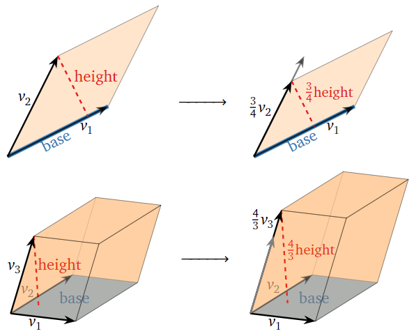
Now , suppose the next row operation consists of multiplying a row by a constant \(k\). For simplicity, we consider a row scaling of the form \(kR_n -> R_n.\) This scales the length of \(\vec{v}_n\) by a factor of \(|k|\text{,}\) which also scales the perpendicular distance of \(\vec{v}_n\) from the base by a factor of \(|k|\). Thus, the volume of the resulting parallelepiped is scaled by \(|k|\), as is the determinant of the matrix made with the tranformed vectors as rows. >
Figure \(\PageIndex{6}\): A diagram illustrating the effect of row scaling on area and volume in linear algebra. In the top row, two parallelograms are shown. On the left, a parallelogram is spanned by vectors \( \vec{v}_1 \) and \( \vec{v}_2 \), where \( \vec{v}_1 \) is labeled as the "base" in blue, and a red dashed line represents the "height" perpendicular to it. On the right, the vector \( v_2 \) is scaled by \( \frac{3}{4} \), reducing the height proportionally to \( \frac{3}{4} \) of its original value. This transformation illustrates that scaling a vector changes the determinant by the same factor. In the bottom row, two parallelepipeds are shown. On the left, the parallelepiped is defined by vectors \( \vec{v}_1, \vec{v}_2, \) and \( \vec{v}_3 \), where \( \vec{v}_1 \) and \( \vec{v}_2 \) form the "base" (shaded in gray), and a red dashed line represents the "height" along \( \vec{v}_3 \). On the right, the vector \( \vec{v}_3 \) is scaled by \( \frac{4}{3} \), increasing the height proportionally to \( \frac{4}{3} \) of its original value. This transformation illustrates that scaling a vector changes the volume by the same factor. (CC-BY-SA; Margalit and Rabinoff via Interactive Linear Algebra)
Now, suppose the next row operation consists of adding a multiple of one row to another. For simplicity, we consider a row replacement of the form \( R_n + cR_i -> R_n\). The volume of a parallelepiped is the volume of its base, times its height: Here the “base” is the parallelepiped determined by \(\vec{v}_1,\vec{v}_2,\ldots,\vec{v}_{n-1}\text{,}\) and the “height” is the perpendicular distance of \(\vec{v}_n\) from the base. Translating \(\vec{v}_n\) by a multiple of \(\vec{v}_i\) moves \(\vec{v}_n\) in a direction parallel to the base. This changes neither the base nor the height! Thus, the volume of the parallelepiped is unchanged by row replacements. And as we know from before, this row operation keeps the determinant of the matrix made of the updated rows unchanged.
Figure \(\PageIndex{7}\): A diagram demonstrating the invariance of area and volume under row operations. In the top row, two parallelograms are shown. On the left, a parallelogram is spanned by vectors \( \vec{v}_1 \) and \( \vec{v}_2 \), where \( \vec{v}_1 \) is labeled as the "base" in blue, and a red dashed line represents the "height" perpendicular to it. On the right, the parallelogram undergoes a row operation where \( \vec{v}_2 \) is replaced by \( \vec{v}_2 - 0.5 \vec{v}_1 \), but the height remains unchanged, preserving the area. In the bottom row, two parallelepipeds are shown. On the left, the parallelepiped is defined by vectors \( \vec{v}_1, \vec{v}_2, \) and \( \vec{v}_3 \), where \( \vec{v}_1 \) and \( \vec{v}_2 \) form the "base" (shaded in gray), and a red dashed line represents the "height" along \( \vec{v}_3 \). On the right, after the row operation \( \vec{v}_3 \to \vec{v}_3 + 0.5 \vec{v}_1 \), the height remains the same, illustrating that the volume is preserved. (CC-BY-SA; Margalit and Rabinoff via Interactive Linear Algebra)
As we can see, the effect of performing elementary row operations on \(I_n\) is identical on the volume of the parallelepiped and the absolute value of the determinant. Hence,
\[|\det(A)| = \text{vol}(P). \nonumber \]
Note
Since \(\det(A) = \det(A^T)\), the absolute value of \(\det(A)\) is also equal to the volume of the parallelepiped determined by the columns of \(A\) as well.
Example \(\PageIndex{4}\): Length
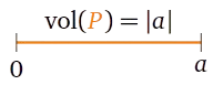
A \(1\times 1\) matrix \(A\) is just a number \(\left(\begin{array}{c}a\end{array}\right)\). In this case, the parallelepiped \(P\) determined by its one row is just the interval \([0,a]\) (or \([a,0]\) if \(a\lt0\)). The “volume” of a region in \(\mathbb{R}^1 = \mathbb{R}\) is just its length, so it is clear in this case that \(\text{vol}(P) = |a|\).
Figure \(\PageIndex{8}\): A diagram illustrating the volume (length) of a one-dimensional interval. A horizontal orange line segment extends from \( 0 \) to \( a \), with vertical bars at both endpoints. Above the segment, the equation \( \text{vol}(P) = |a| \) is displayed, indicating that the length of the interval is given by the absolute value of \( a \). The endpoints are labeled \( 0 \) and \( a \), representing the interval's boundaries. (CC-BY-SA; Margalit and Rabinoff via Interactive Linear Algebra)
Example \(\PageIndex{5}\): Area
When \(A\) is a \(2\times 2\) matrix, its rows determine a parallelogram in \(\mathbb{R}^2 \). The “volume” of a region in \(\mathbb{R}^2 \) is its area, so we obtain a formula for the area of a parallelogram: it is the determinant of the matrix whose rows are the vectors forming two adjacent sides of the parallelogram.
Figure \(\PageIndex{9}\): A diagram illustrating the area of a parallelogram using the determinant. On the left, a parallelogram is shown in a two-dimensional plane, defined by two black vectors originating from a common point. These vectors are labeled as column vectors \( \begin{pmatrix} a \\ b \end{pmatrix} \) and \( \begin{pmatrix} c \\ d \end{pmatrix} \). The parallelogram is shaded in light orange. On the right, the formula for the area of the parallelogram is displayed: \( \text{area} = \left| \det \begin{pmatrix} a & b \\ c & d \end{pmatrix} \right| = |ad - bc| \) which shows that the absolute value of the determinant of the matrix formed by the two vectors gives the area of the parallelogram. This diagram visually demonstrates how the determinant provides a measure of area in two dimensions. (CC-BY-SA; Margalit and Rabinoff via Interactive Linear Algebra)
It is perhaps surprising that it is possible to compute the area of a parallelogram without trigonometry. It is a fun geometry problem to prove this formula by hand. [Hint: first think about the case when the first row of \(A\) lies on the \(x\)-axis.]
Example \(\PageIndex{6}\)
Find the area of the parallelogram with sides \((1,3)\) and \((2,-3)\).
Figure \(\PageIndex{10}\): A parallelogram plotted on a coordinate grid, defined by two black arrows representing vectors originating from a common point. The parallelogram is shaded in light orange, illustrating the region whose area is determined by the determinant of the matrix formed by the vectors. The grid provides a reference for the positioning of the parallelogram in two-dimensional space. (CC-BY-SA; Margalit and Rabinoff via Interactive Linear Algebra)
Find the area of the parallelogram in the picture.
Figure \(\PageIndex{11}\): A parallelogram plotted on a coordinate grid. The points are not labeled. Starting with the top-left point as the first point and moving clockwise, the second point is 2 units right and 1 unit down from the first point. The third point is 1 unit left and 4 units down from the second point. The fourth point is 2 units left and 1 unit up from the third point. The first point is 1 unit right and 4 units up from the fourth point. (CC-BY-SA; Margalit and Rabinoff via Interactive Linear Algebra)
Solution
We choose two adjacent sides to be the rows of a matrix. We choose the top two:
Figure \(\PageIndex{12}\): A parallelogram plotted on a coordinate grid, defined by two vectors originating from a common point (the top-left point of the parallelogram). The vectors are labeled with their components: \( \begin{pmatrix} -1 \\ -4 \end{pmatrix} \) and \( \begin{pmatrix} 2 \\ -1 \end{pmatrix} \). (CC-BY-SA; Margalit and Rabinoff via Interactive Linear Algebra)
Note that we do not need to know where the origin is in the picture: vectors are determined by their length and direction, not where they start. The area is
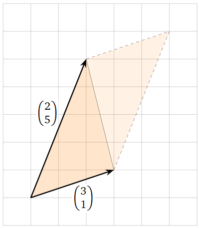
Find the area of the triangle with vertices \((-1,-2), \,(2,-1),\,(1,3).\)
Figure \(\PageIndex{13}\): A triangle plotted on a coordinate grid. The triangle is formed by three points, creating a geometric region in two-dimensional space. The points are not labeled. Starting with the bottom-left point as the first point and moving clockwise, the second point is 2 units right and 5 units up. The third point is 1 unit right and 4 units down from the second point. The first point is 3 units left and 1 unit down from the third point. (CC-BY-SA; Margalit and Rabinoff via Interactive Linear Algebra)
Solution
Doubling a triangle makes a parallelogram. We choose two of its sides to be the rows of a matrix.
Figure \(\PageIndex{14}\): A triangle given in the example is extended to a parallelogram defined by two vectors originating from a common point. The vectors are labeled with their components: \( \begin{pmatrix} 2 \\ 5 \end{pmatrix} \) and \( \begin{pmatrix} 3 \\ 1 \end{pmatrix} \). The original triangle is shaded darker than the triangle added to form the parallelogram. (CC-BY-SA; Margalit and Rabinoff via Interactive Linear Algebra)
You might be wondering: if the absolute value of the determinant is a volume, what is the geometric meaning of the determinant without the absolute value? The next remark explains that we can think of the determinant as a signed volume. If you have taken an integral calculus course, you probably computed negative areas under curves; the idea here is similar.
Remark: Signed volumes
Theorem \(\PageIndex{1}\) on determinants and volumes tells us that the absolute value of the determinant is the volume of a paralellepiped. This raises the question of whether the sign of the determinant has any geometric meaning.
A \(1\times 1\) matrix \(A\) is just a number \(\left(\begin{array}{c}a\end{array}\right)\). In this case, the parallelepiped \(P\) determined by its one row is just the interval \([0,a]\) if \(a \geq 0\text{,}\) and it is \([a,0]\) if \(a\lt0\). In this case, the sign of the determinant determines whether the interval is to the left or the right of the origin.
For a \(2\times 2\) matrix with rows \(v_1,v_2\text{,}\) the sign of the determinant determines whether \(v_2\) is counterclockwise or clockwise from \(v_1\). That is, if the counterclockwise angle from \(v_1\) to \(v_2\) is less than \(180^\circ\text{,}\) then the determinant is positive; otherwise it is negative (or zero).
Figure \(\PageIndex{15}\): A comparison of two parallelograms, each defined by two vectors, \( \vec{v}_1 \) and \( \vec{v}_2 \), originating from a common point. On the left, the parallelogram is oriented such that the determinant of the matrix formed by \( \vec{v}_1 \) and \(\vec{v}_2 \) is positive, indicated by the expression: \(\det \begin{pmatrix} \vec{v}_1 & \vec{v}_2 \end{pmatrix} > 0.\) A signed angle between the vectors is shown and is positive, emphasizing their orientation. On the right, the parallelogram is oriented in the opposite way, resulting in a negative determinant: \( \det \begin{pmatrix} \vec{v}_1 & \vec{v}_2 \end{pmatrix} < 0. \) The reversed orientation demonstrates the effect of swapping the vectors on the determinant's sign. (CC-BY-SA; Margalit and Rabinoff via Interactive Linear Algebra)
For example, if \(v_1 = {a\choose b}\text{,}\) then the counterclockwise rotation of \(v_1\) by \(90^\circ\) is \(v_2 = {-b\choose a}\) by Example 3.3.8 in Section 3.3, and
For a \(3\times 3\) matrix with rows \(v_1,v_2,v_3\text{,}\) the right-hand rule determines the sign of the determinant. If you point the index finger of your right hand in the direction of \(v_1\) and your middle finger in the direction of \(v_2\text{,}\) then the determinant is positive if your thumb points roughly in the direction of \(v_3\text{,}\) and it is negative otherwise.
Figure \(\PageIndex{16}\): A comparison of two three-dimensional parallelepipeds, each defined by three vectors, \( \vec{v}_1 \), \( \vec{v}_2 \), and \( \vec{v}_3 \), originating from a common point. On the left, the parallelepiped is oriented such that the determinant of the matrix formed by \( \vec{v}_1 \), \( \vec{v}_2 \), and \( \vec{v}_3 \) is positive, indicated by the expression: \( \det \begin{pmatrix} \vec{v}_1 & \vec{v}_2 & \vec{v}_3 \end{pmatrix} > 0. \) The vectors are labeled and shown extending from a common vertex. On the right, the parallelepiped is oriented differently, resulting in a negative determinant: \(\det \begin{pmatrix} \vec{v}_1 & \vec{v}_2 & \vec{v}_3 \end{pmatrix} < 0. \) The reversed orientation demonstrates the effect of changing the order of the vectors on the determinant's sign. (CC-BY-SA; Margalit and Rabinoff via Interactive Linear Algebra)
In higher dimensions, the notion of signed volume is still important, but it is usually defined in terms of the sign of a determinant.