11.2: The Density Curve of a Normal Distribution

Last updated
Save as PDF

Page ID: 109922

$ \newcommand{\vecs}[1]{\overset { \scriptstyle \rightharpoonup} {\mathbf{#1}} } $ $ \newcommand{\vecd}[1]{\overset{-\!-\!\rightharpoonup}{\vphantom{a}\smash {#1}}} $$\newcommand{\id}{\mathrm{id}}$ $ \newcommand{\Span}{\mathrm{span}}$ $ \newcommand{\kernel}{\mathrm{null}\,}$ $ \newcommand{\range}{\mathrm{range}\,}$ $ \newcommand{\RealPart}{\mathrm{Re}}$ $ \newcommand{\ImaginaryPart}{\mathrm{Im}}$ $ \newcommand{\Argument}{\mathrm{Arg}}$ $ \newcommand{\norm}[1]{\| #1 \|}$ $ \newcommand{\inner}[2]{\langle #1, #2 \rangle}$ $ \newcommand{\Span}{\mathrm{span}}$ $\newcommand{\id}{\mathrm{id}}$ $ \newcommand{\Span}{\mathrm{span}}$ $ \newcommand{\kernel}{\mathrm{null}\,}$ $ \newcommand{\range}{\mathrm{range}\,}$ $ \newcommand{\RealPart}{\mathrm{Re}}$ $ \newcommand{\ImaginaryPart}{\mathrm{Im}}$ $ \newcommand{\Argument}{\mathrm{Arg}}$ $ \newcommand{\norm}[1]{\| #1 \|}$ $ \newcommand{\inner}[2]{\langle #1, #2 \rangle}$ $ \newcommand{\Span}{\mathrm{span}}$$\newcommand{\AA}{\unicode[.8,0]{x212B}}$

Learning Objectives

Identify the properties of a normal density curve and the relationship between concavity and standard deviation.
Convert between z-scores and areas under a normal probability curve.
Calculate probabilities that correspond to left, right, and middle areas from a z-score table.
Calculate probabilities that correspond to left, right, and middle areas using a graphing calculator.
Calculate for unknown values other than the z-score and area.

Introduction

In this section, we will continue our investigation of normal distributions to include density curves and learn various methods for calculating probabilities from the normal density curve.

Density Curves

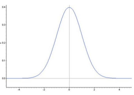
A density curve is an idealized representation of a distribution in which the area under the curve is defined to be 1. Density curves need not be normal, but the normal density curve will be the most useful to us.

$clipboard_e55debb140b50395d23f02df4f6532705.png$

Inflection Points on a Normal Density Curve

We already know from the Empirical Rule that approximately $\dfrac{2}{3}$ of the data in a normal distribution lies within 1 standard deviation of the mean. With a normal density curve, this means that about 68% of the total area under the curve is within z-scores of $±1$. Look at the following three density curves:

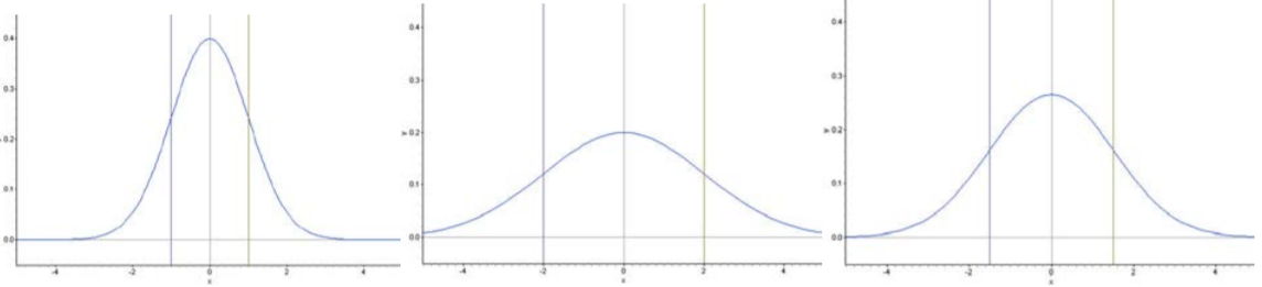
$clipboard_e2fda7c72c9da7175992992365a4d325c.png$

Notice that the curves are spread increasingly wider. Lines have been drawn to show the points that are one standard deviation on either side of the mean. Look at where this happens on each density curve.

Here is a normal distribution with an even larger standard deviation.

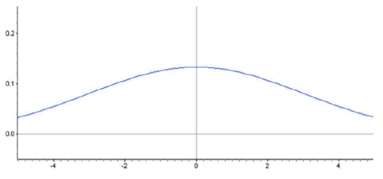
$clipboard_ec49ac19b24a9565677c2c92d614d1b26.png$

Is it possible to predict the standard deviation of this distribution by estimating the $x$-coordinate of a point on the density curve? Read on to find out!

You may have noticed that the density curve changes shape at two points in each of our examples. These are the points where the curve changes concavity. Starting from the mean and heading outward to the left and right, the curve is concave down. (It looks like a mountain, or ‘$n$’ shape.) After passing these points, the curve is concave up. (It looks like a valley, or ‘$u$’ shape.) The points at which the curve changes from being concave up to being concave down are called the inflection points. On a normal density curve, these inflection points are always exactly one standard deviation away from the mean.

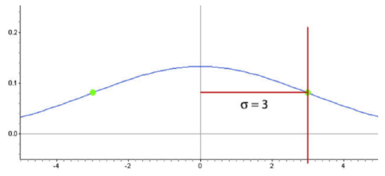
$clipboard_e2388c90c4abe165bfd76d30d9698c7d7.png$

In this example, the standard deviation is 3 units. We can use this concept to estimate the standard deviation of a normally distributed data set.

Example $\PageIndex{1}$

Estimate the standard deviation of the distribution represented by the following histogram.

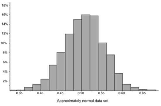
$clipboard_e79fd6fd1a0942641cf432f6da1e6b623.png$

Solution

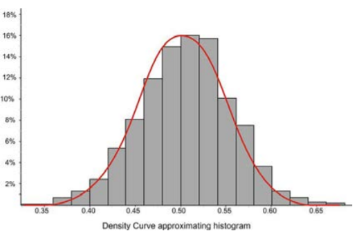
This distribution is fairly normal, so we could draw a density curve to approximate it as follows:

$clipboard_e9ae06771dc0008ac38f370117bcc7c37.png$

Now estimate the inflection points as shown below:

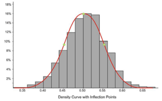
$clipboard_e5e82ab30b1d03737849dd79fa39853bc.png$

It appears that the mean is about 0.5 and that the $x$-coordinates of the inflection points are about 0.45 and 0.55, respectively. This would lead to an estimate of about 0.05 for the standard deviation.

The actual statistics for this distribution are as follows:

$s ≈ 0.04988$

$\overline{x} ≈ 0.4997$

We can verify these figures by using the expectations from the Empirical Rule. In the following graph, we have highlighted the bins that are contained within one standard deviation of the mean.

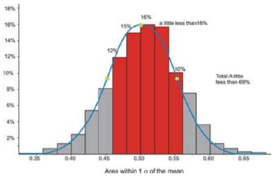
$clipboard_e358399bfbe569b52330fcf02930cd484.png$

If you estimate the relative frequencies from each bin, their total is remarkably close to 68%. Make sure to divide the relative frequencies from the bins on the ends by 2 when performing your calculation.

Convert Between z-scores and Areas

While it is convenient to estimate areas under a normal curve using the Empirical Rule, we often need more precise methods to calculate these areas. Luckily, we can use formulas or technology to help us with the calculations.

z-scores

All normal distributions have the same basic shape, and therefore, rescaling and re-centering can be implemented to change any normal distributions to one with a mean of 0 and a standard deviation of 1. This configuration is referred to as a standard normal distribution. In a standard normal distribution, the variable along the horizontal axis is the z-score. This score is another measure of the performance of an individual score in a population. To review, the z-score measures how many standard deviations a score is away from the mean. The z-score of the term $x$ in a population distribution whose mean is $µ$ and whose standard deviation is $σ$ is given by: $\dfrac{x-µ}{σ}$. Since $σ$ is always positive, $z$ will be positive when $x$ is greater than $µ$ and negative when $x$ is less than $µ$. A z-score of $0$ means that the term has the same value as the mean. The value of $z$ is the number of standard deviations the given value of $x$ is above or below the mean.

Example $\PageIndex{2}$

On a nationwide math test, the mean was 65 and the standard deviation was 10. If Robert scored 81, what was his z-score?

Solution

$z = \dfrac{x-µ}{σ}$

$z = \dfrac{81-65}{1.6}$

$z = 10$

Example $\PageIndex{3}$

On a college entrance exam, the mean was 70 and the standard deviation was 8. If Helen’s z-score was −1.5, what was her exam score?

Solution

Recall, the equation to obtain $x$ is

$x = µ +zσ$

Using this equation, we can find Helen’s score:

$x = µ +zσ$

$x = 70 +(-1.5)(8)$

$x = 58$

Now you will see how z-scores are used to determine the probability of an event.

Example $\PageIndex{4}$

Suppose you were to toss 8 coins 256 times. The following figure shows the histogram and the approximating normal curve for the experiment. The random variable represents the number of tails obtained.

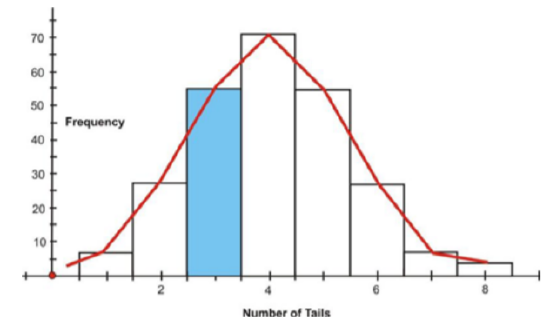
$clipboard_ea6f1c576e8c9b3c087ab9de0139bb301.png$

The blue section of the graph represents the probability that exactly 3 of the coins turned up tails. Geometrically, this probability represents the area of the blue shaded bar divided by the total area of the bars. The area of the blue shaded bar is approximately equal to the area under the normal curve from 2.5 to 3.5.

Since areas under normal curves correspond to the probability of an event occurring, a special normal distribution table is used to calculate the probabilities. This table can be found at the end of this section where the area is given from the mean. The following is an example of a table of z-scores and a brief explanation of how it works: http://tinyurl.com/2ce9ogv.

The values inside the given table represent the areas under the standard normal curve for values between 0 and the relative z-score. For example, to determine the area under the curve between zscores of 0 and 2.36, look in the intersecting cell for the row labeled 2.3 and the column labeled 0.06. The area under the curve is 0.4909. To determine the area between 0 and a negative value, look in the intersecting cell of the row and column which sums to the absolute value of the number in question. For example, the area under the curve between −1.3 and 0 is equal to the area under the curve between 1.3 and 0, so look at the cell that is the intersection of the 1.3 row and the 0.00 column. (The area is 0.4032.)

Calculate Probabilities that Correspond to z-scores and Areas

It is extremely important, especially when you first start with these calculations, that you get in the habit of relating it to the normal distribution by drawing a sketch of the situation. In this case, simply draw a sketch of a standard normal curve with the appropriate region shaded and labeled.

$clipboard_e1b837635dfe4481b2c5ec2e115fae7cf.png$

Example $\PageIndex{5}$

Find the probability of choosing a value that is greater than $z = −0.528$, or $P(z > −0.528)$.

Solution

Before even using the table, first draw a figure with the shaded region. This z-score is just below the mean, so the answer should be more than 0.5.

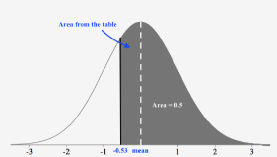
$clipboard_e004dd255a98a67e325ae735bc55db0d5.png$

Next, read the table to find the correct probability for the data below this z-score. We must first round this z-score to −0.53, so this will slightly under-estimate the probability, but it is the best we can do using the table. Looking up a z-score of −0.53, we see

z	0.00	0.01	0.02	0.03
0.00	0.00000	0.00399	0.00798	0.01197
0.10	0.03983	0.04380	0.04776	0.05172
0.20	0.07926	0.08317	0.08706	0.09095
0.30	0.11791	0.12712	0.12552	0.12930
0.40	0.15542	0.15910	0.16276	0.16640
0.50	0.19146	0.19497	0.19847	0.20194

The table returns an area of 0.20194. Since the area from the mean to $z = −0.53$ is $0.20194$ and the area on the right of the mean is 0.5, then the area of the shaded region is

$0.5 + 0.20194 = 0.70194$

Thus, the probability of choosing a value that is greater than $z = −0.528$ is $0.7019$.

What about values between two z-scores? While it is an interesting and worthwhile exercise to do this using a table, we can also use statistical software or a graphing calculator.

Example $\PageIndex{6}$

Find $P(−2.60 < z < 1.30)$.

Solution

First, we draw a figure with the shaded region:

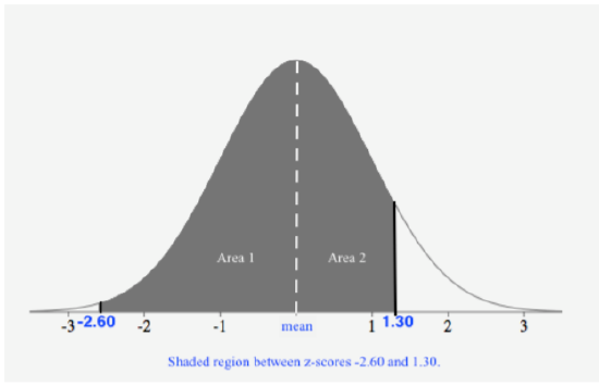
$clipboard_e1876142893d20ed7f63f141e029826a8.png$

Since the table gives us the area from the mean to a z-score, we can see that we will add the areas, Area 1 + Area 2, to obtain the area of the shaded region, resulting in the probability. Let’s look up the z-scores on the table to find the area from the mean to each z-score:

z	0.00
1.30	0.40320
2.60	0.49534

Area 1 is $0.49534$ and Area 2 is $0.40320$. Adding these two together, we get

$P(−2.60 < z < 1.30)= \text{ Area } 1 + \text{ Area } 2 = 0.49534 + 0.40320 = 0.89854$

Thus, the probability $P(−2.60 < z < 1.30) = 0.89854$.

The probability can also be found using the TI-83/84 calculator. Use the ‘normalcdf(−2.60, 1.30, 0, 1)’ command, and the calculator will return the result 0.898538. The syntax for this command is ‘normalcdf(min, max, µ, σ)’. When using this command, you do not need to first standardize. You can use the mean and standard deviation of the given distribution.

Technology Note: The 'normalcdf(' Command on TI-83/84 Calculator

Your graphing calculator has already been programmed to calculate probabilities for a normal density curve using what is called a cumulative density function. The command you will use is found in the DISTR menu, which you can bring up by pressing [2ND][DISTR].

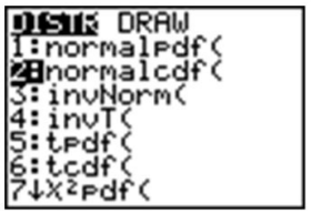
$clipboard_e1e131e3ffe96383fe61d470adda38b12.png$

Press [2] to select the ‘normalcdf(’ command, which has a syntax of ‘normalcdf(lower bound, upper bound, mean, standard deviation)’.

The command has been programmed so that if you do not specify a mean and standard deviation, it will default to the standard normal curve, with $µ = 0$ and $σ = 1$.

For example, entering ‘normalcdf(−1, 1)’ will specify the area within one standard deviation of the mean, which we already know to be approximately 0.68.

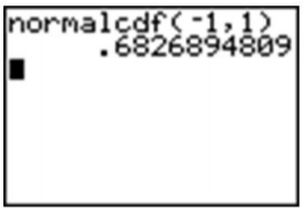
$clipboard_ebee14d8a33c8b08ec6a421546f371b8d.png$

Try verifying the other values from the Empirical Rule.

Summary:

‘Normalcdf ($a,b,µ,σ$)’ gives values of the cumulative normal density function. In other words, it gives the probability of an event occurring between $x = a$ and $x = b$, or the area under the probability density curve between the vertical lines $x = a$ and $x = b$, where the normal distribution has a mean of $µ$ and a standard deviation of $σ$. If $µ$ and $σ$ are not specified, it is assumed that $µ = 0$ and $σ = 1$.

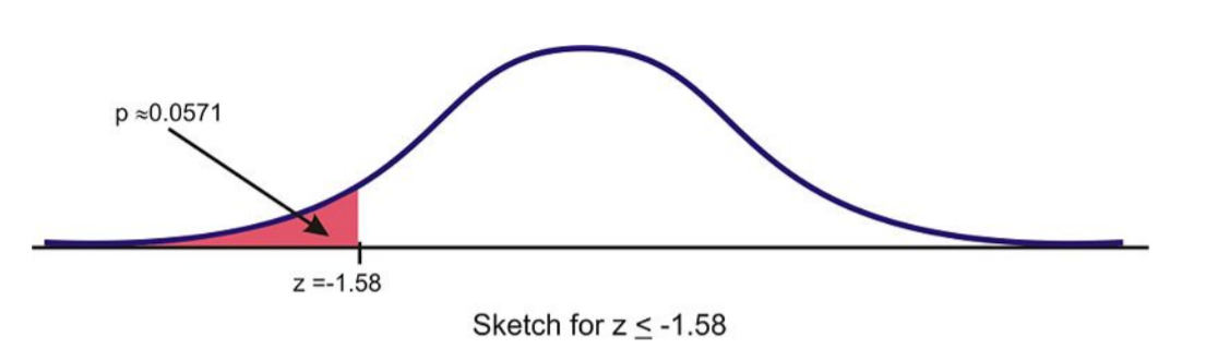
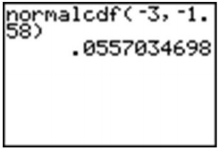
$clipboard_e9065415bcb545b719ba18019fa7ea1ba.png$

Example $\PageIndex{7}$

Find the probability $P(z < −1.58)$.

Solution

First, we draw a figure with the shaded region:

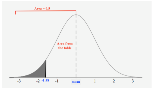
$clipboard_ed4311ba32e5808b8dd306b6e5f9dfcd3.png$

Since the table gives us the area from the mean to a z-score and the total area to the left of the mean is 0.5, we can see that we will subtract the area given in the table from 0.5 to obtain the area of the shaded region, resulting in the probability. Let’s look up the z-score on the table to find the area from the mean to the z-score:

z	0.08
1.50	0.44295

The area from the mean to $z = –1.58$ is $0.44295$. Subtracting this from $0.5$, we get

$P(z < −1.58) = 0.5 – 0.44295 = 0.05705$

Doing this on the calculator, we must have both an upper and lower bound. Technically, though, the density curve does not have a lower bound, as it continues infinitely in both directions. We do know, however, that a very small percentage of the data is below 3 standard deviations to the left of the mean. Use −3 as the lower bound and see what answer you get.

$clipboard_e93418cbcbc3f3c9f5b73dc080cadf4af.png$

The answer is fairly accurate, but you must remember that there is really still some area under the probability density curve, even though it is just a little, that we are leaving out if we stop at −3. If you look at the z-table, you can see that we are, in fact, leaving out about $0.5 − 0.4987 = 0.0013$. Next, try going out to −4 and −5.

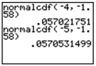
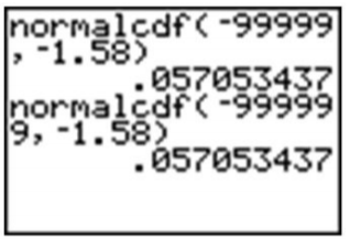
$clipboard_e4b1b8abe9d92e426543b7d8d57f69010.png$

Once we get to −5, the answer is quite accurate. Since we cannot really capture all the data, entering a sufficiently small value should be enough for any reasonable degree of accuracy. A quick and easy way to handle this is to enter −99999 (or “a bunch of nines”). It really doesn’t matter exactly how many nines you enter. The difference between five and six nines will be beyond the accuracy that even your calculator can display.

$clipboard_e4bb7f8e9f43ac2d9b2867f51bbc5ada3.png$

Example $\PageIndex{8}$

Find the probability $P(0 < z < 1.78)$.

Solution

First, we draw a figure with the shaded region:

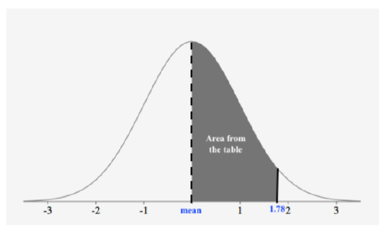
$clipboard_e7c587ff8d8d91a942383d59dcd485e15.png$

Since the table gives us the area from the mean to a z-score, we can see that whatever area is given from the table results in the probability. Let’s look up the z-score on the table to find the area from the mean to the z-score.

z	0.08
1.70	0.46246

The area from the mean to $z = 1.78$ is $0.46246$. Thus,

$P(z < 1.78) = 0.46246$

We are at an advantage using the calculator because we do not have to round off the z-score in this example. Let’s try this example with the calculator. Enter the ‘normalcdf(’ command, using −0.528 to “a bunch of nines.” The nines represent a ridiculously large upper bound that will insure that the unaccounted-for probability will be so small that it will be virtually undetectable.

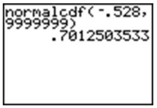
$clipboard_e22bbc1dee9da31bc6e998b90b55232d8.png$

Remember that because of rounding, our answer from the table was slightly too small, so when we subtracted it from $1$, our final answer was slightly too large. The calculator answer of about $0.70125$ is a more accurate approximation than the answer arrived at by using the table.

Standardizing

In most practical problems involving normal distributions, the curve will not be as we have seen so far, with $µ = 0$ and $σ = 1$. When using a z-table, you will first have to standardize the distribution by calculating the z-score(s).

Example $\PageIndex{9}$

A candy company sells small bags of candy and attempts to keep the number of pieces in each bag the same, though small differences due to random variation in the packaging process lead to different amounts in individual packages. A quality control expert from the company has determined that the mean number of pieces in each bag is normally distributed, with a mean of 57.3 and a standard deviation of 1.2. Endy opened a bag of candy and felt he was cheated. His bag contained only 55 candies. Does Endy have reason to complain?

Solution

To determine if Endy was cheated, we need to find the probability of selecting a bag of candy with 55 or fewer candies, i.e., we let $x = 55$. Let’s calculate the z-score for 55:

$z = \dfrac{x-µ}{σ}$

$z = \dfrac{55-57.3}{1.2}$

$z ≈ -1.91$

Next, we can draw a figure to see the shaded region:

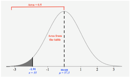
$clipboard_e2041b491f7d5dea24f16945fc398ccfa.png$

Using a table, we obtain a value $0.47193$. This is the area from the mean to $z = −1.91$. We can subtract this value from $0.5$ since the area on the left of the mean is $0.5$:

$0.5 − 0.47193 = 0.02807$

Hence, there is about a 3% chance that he would get a bag of candy with 55 or fewer pieces, so Endy should feel cheated because the chances of getting a bag with 55 or fewer candies is so low.

Using a graphing calculator, the results would look as follows (the ‘Ans’ function has been used to avoid rounding off the z-score):

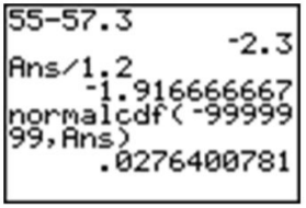
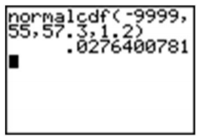
$clipboard_e635fa728e0ab5268cfa5a082a59440e1.png$

However, one of the advantages of using a calculator is that it is unnecessary to standardize. We can simply enter the mean and standard deviation from the original population distribution of candy, avoiding the z-score calculation completely.

$clipboard_e3db571289c26f7fc32059b5e23b79348.png$

Unknown Value Problems

If you understand the relationship between the area under a density curve and mean, standard deviation, and z-scores, you should be able to solve problems in which you are provided all but one of these values and are asked to calculate the remaining value. In the last lesson, we found the probability that a variable is within a particular range, or the area under a density curve within that range. What if you are asked to find a value that gives a particular probability? We rewrite the z-score formula $z = \dfrac{x-µ}{σ}$ as

$x = µ +z \cdot σ\;\;\; \text{ or }\;\;\; µ = x - z \cdot σ$

Unknown Original Value, $x$

Example $\PageIndex{10}$

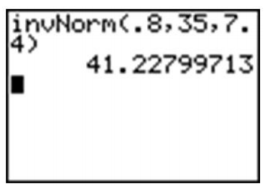
Given the normally-distributed random variable $x$, with $µ = 35$ and $σ = 7.4$, what is the value of $x$ where the probability of experiencing a value less than it is 80%?

Solution

As suggested before, it is important and helpful to sketch the distribution.

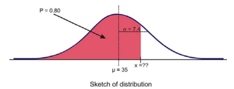
$clipboard_e42cd22ccb903fd23af94928cd762f58b.png$

We need to find a z-score from the table that corresponds to the area from the mean. Since the area on the left of the mean is $0.5$, we see that the area from the mean to $x$ is $0.30$, i.e.,

$P(z < x) = 0.8$

and this implies that

$P(0 < z < x) = 0.8 − 0.5 = 0.3$

We need to find, somewhere in the areas given in the table, an area of $0.3$ (or the closest to it) and its corresponding z-score. Let’s take a look:

z	0.04	0.05
0.80	0.29955	0.30234

We see the closest area to $0.3$, given in the table, is $0.29955$, which has a corresponding z-score of $0.84$. Hence, we use $z = 0.84$ for the z-score in the formula to obtain $x$. Given $µ = 35$ and $σ = 7.4$, we get

$x = µ +z \cdot σ$

$x = 35 + 0.84(7.4)$

$x = 41.216$

Thus, the value of $x$ where the probability of experiencing a value less than it is $80 \% $ is $41.216$. In general, when we want to obtain an $x$ value from a given probability, we find the z-score first, then plug-n-chug this into the rewritten z-score formula.

When we were given a value of the variable and were asked to find the percentage or probability, the ‘normalcdf(’ command on a graphing calculator. But how do we find a value given the percentage? Graphing calculators and computer software are much more convenient and accurate. The command on the TI-83/84 calculator is ‘invNorm(’. You may have seen it already in the DISTR menu.

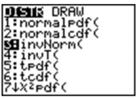
$clipboard_efb4b725fc1137074a07f0189bbe1ff20.png$

The syntax for this command is as follows:

‘InvNorm(percentage or probability to the left, mean, standard deviation)’

Make sure to enter the values in the correct order, such as in the example below:

$clipboard_e6c16dbf2d9feedb942a99ec40b2facb2.png$

Unknown Mean or Standard Deviation

Example $\PageIndex{11}$

For a normally distributed random variable, $σ = 4.5$, $x = 20$, and $P = 0.05$, find $.$

Solution

To solve this problem, first draw a sketch:

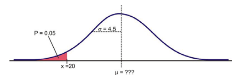
$clipboard_ee5d08aa93f6165ce894b70e6015c1f12.png$

We need to find a z-score from the table that corresponds to the area from the mean. Since the area on the left of $x = 20$ is $0.05$, we see that the area from the mean to $x$ is $0.45$, i.e.,

$P(z < x) = 0.05$

and this implies that

$P(x < z < 0) = 0.5 − 0.05 = 0.45$

We need to find, somewhere in the areas given in the table, an area of $0.45$ (or the closest to it) and its corresponding negative z-score, since the $x$ value lies below the mean. Let’s take a look:

z	0.04	0.05
1.60	0.44950	0.45953

We see the closest area to $0.45$, given in the table, is $0.44950$, which has a corresponding z-score of $-1.64$. Recall, the z-score is negative because the x value lies below the mean. Hence, we use $z = −1.64$ for the z-score in the formula to obtain $x$. Given $σ = 4.5$ and $x = 20$, we get

$µ = x-z \cdot σ$

$µ = 20 - (-1.64)(4.5)$

$µ = 41.216$

Thus, the mean is $27.38$.

We could also use the ‘invNorm(’ command on the calculator. The result, $−1.645$, confirms the prediction that the value is less than 2 standard deviations from the mean.

Now, plug in the known quantities into the z-score formula and solve for $µ$ as follows:

$z = \dfrac{x - µ}{σ}$

$µ = x-zσ$

$µ ≈ 20 - (-1.645)(4.5)$

$z ≈ 27.402$

We can see there was little discrepancy from using the table and using the calculator. However, since we were eye-balling from the table, the calculator gives more accurate results.

Example $\PageIndex{12}$

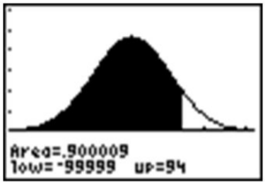
For a normally-distributed random variable, $µ = 83$, $x = 94$, and $P = 0.90$. Find $σ$.

Solution

Again, let’s first look at a sketch of the distribution.

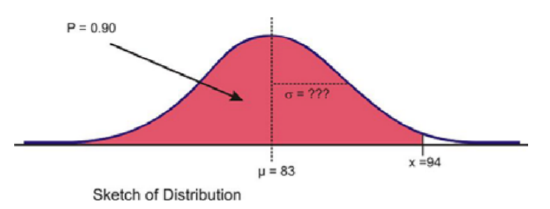
$clipboard_e1cc3894a0721dc0e392f1244fb7da4a2.png$

Since about 97.5% of the data is below 2 standard deviations, it seems reasonable to estimate that the $x$ value is less than two standard deviations away from the mean and that $σ$ might be around $7$ or $8$.

Again, the first step to see if our prediction is right is to use ‘invNorm(’ to calculate the z-score. Remember that since we are not entering a mean or standard deviation, the result is based on the assumption that $µ = 0$ and $σ = 1$.

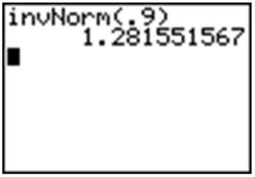
$clipboard_e58261ff274f8f66cf3421559744be609.png$

Now, use the z-score formula and solve for $σ$ as follows:

$z = \dfrac{x - µ}{σ}$

$σ = \dfrac{x - µ}{z}$

$σ = \dfrac{94 - 83}{1.282}$

$σ ≈ 8.583 $

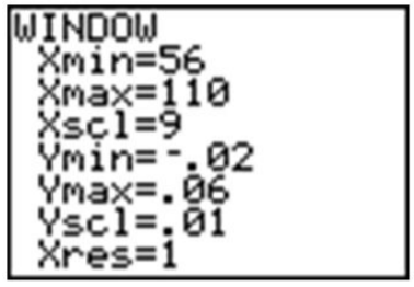
Technology Note: Drawing a Distribution on the TI-83/84 Calculator

The TI-83/84 calculator will draw a distribution for you, but before doing so, we need to set an appropriate window (see screen below) and delete or turn off any functions or plots. Let’s use the last example and draw the shaded region below $94$ under a normal curve with $µ = 83$ and $σ = 8.583$. Remember from the Empirical Rule that we probably want to show about $3$ standard deviations away from $83$ in either direction. If we use $9$ as an estimate for $σ$, then we should open our window $27$ units above and below $83$. The $y$ settings can be a bit tricky, but with a little practice, you will get used to determining the maximum percentage of area near the mean.

$clipboard_e22d450ef80838dfaee66b81ea1927040.png$

The reason that we went below the x-axis is to leave room for the text, as you will see.

Now, press [2ND][DISTR] and arrow over to the DRAW menu.

Choose the ‘ShadeNorm(’ command. With this command, you enter the values just as if you were doing a ‘normal cdf(’ calculation. The syntax for the ‘ShadeNorm(’ command is as follows: ‘ShadeNorm(lower bound, upper bound, mean, standard deviation)’

Enter the values shown in the following screenshot:

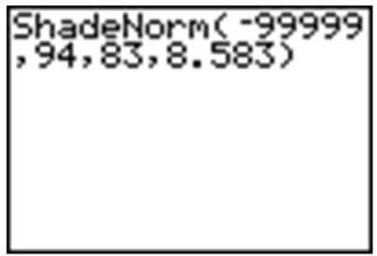
$clipboard_ec926ed0f5feb49b9d1c520ff4d8b6051.png$

Next, press [ENTER] to see the result. It should appear as follows:

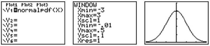
$clipboard_ef9ed79d1cd80e6963db6189762346fdd.png$

Technology Note: The 'normalpdf(' Command on TI-83/84 Calculator

You may have noticed that the first option in the DISTR menu is ‘normalpdf(’, which stands for a normal probability density function. It is the option you used in Lesson 5.1 to draw the graph of a normal distribution. Many students wonder what this function is for and occasionally even use it by mistake to calculate what they think are cumulative probabilities, but this function is actually the mathematical formula for drawing a normal distribution. You can find this formula in the resources at the end of the lesson if you are interested. The numbers this function returns are not really useful to us statistically. The primary purpose for this function is to draw the normal curve.

To do this, first be sure to turn off any plots and clear out any functions. Then press [Y=], insert ‘normalpdf(’, enter ‘X’, and close the parentheses as shown. Because we did not specify a mean and standard deviation, the standard normal curve will be drawn. Finally, enter the following window settings, which are necessary to fit most of the curve on the screen (think about the Empirical Rule when deciding on settings), and press [GRAPH]. The normal curve below should appear on your screen.

$clipboard_e7d17d67c0e250d8721c6183ed50f92a7.png$

Important links: Tables and Calculators

This link leads you to a z-score table and an explanation of how to use it: http://tinyurl.com/2ce9ogv
Here’s a normal distribution calculator. Use this calculator to verify your answers and drawing a figure: http://tinyurl.com/n6uwo5m

Exercises

1. Estimate the standard deviation of the following distribution.

$clipboard_e3ca4fa04416f07a745d934433077ce5c.png$

2. Calculate the following probabilities using only the z-table. Show all your work.

a) $P(z ≥−0.79)$

b) $P(−1 ≤ z ≤ 1)$ Show all work.

c) $P(−1.56 < z < 0.32)$

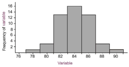
3. Brielle’s statistics class took a quiz, and the results were normally distributed, with a mean of 85 and a standard deviation of 7. She wanted to calculate the percentage of the class that got a B (between 80 and 90). She used her calculator and was puzzled by the result. Here is a screen shot of her calculator:

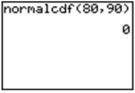
$clipboard_ed3c76e16a3b8c4346b2d18612b6f1275.png$

Explain her mistake and the resulting answer on the calculator, and then calculate the correct answer.

4. Which grade is better: A 78 on a test whose mean is 72 and standard deviation is 6.5, or an 83 on a test whose mean is 77 and standard deviation is 8.4. Justify your answer and draw sketches of each distribution.

5. Teachers A and B have final exam scores that are approximately normally distributed, with the mean for Teacher A equal to 72 and the mean for Teacher B equal to 82. The standard deviation of Teacher A’s scores is 10, and the standard deviation of Teacher B’s scores is 5.

a) With which teacher is a score of 90 more impressive? Support your answer with appropriate probability calculations and with a sketch.

b) With which teacher is a score of 60 more discouraging? Again, support your answer with appropriate probability calculations and with a sketch.

6. For each of the following problems, $X$ is a continuous random variable with a normal distribution and the given mean and standard deviation. $P$ is the probability of a value of the distribution being less than $x$. Find the missing value and sketch and shade the distribution.

Mean	Standard Deviation	$x$	$P$, probability
85	4.5		0.68
	1	16	0.05
73		85	0.91
93	5		0.90

7. What is the z-score for the lower quartile in a standard normal distribution?

Search

Learning Objectives

Introduction

Density Curves

Inflection Points on a Normal Density Curve

Example \(\PageIndex{1}\)

Convert Between z-scores and Areas

z-scores

Example \(\PageIndex{2}\)

Example \(\PageIndex{3}\)

Example \(\PageIndex{4}\)

Calculate Probabilities that Correspond to z-scores and Areas

Example \(\PageIndex{5}\)

Example \(\PageIndex{6}\)

Technology Note: The 'normalcdf(' Command on TI-83/84 Calculator

Example \(\PageIndex{7}\)

Example \(\PageIndex{8}\)

Standardizing

Example \(\PageIndex{9}\)

Unknown Value Problems

Unknown Original Value, \(x\)

Example \(\PageIndex{10}\)

Unknown Mean or Standard Deviation

Example \(\PageIndex{11}\)

Example \(\PageIndex{12}\)

Technology Note: Drawing a Distribution on the TI-83/84 Calculator

Technology Note: The 'normalpdf(' Command on TI-83/84 Calculator

Important links: Tables and Calculators

Exercises

Mean	Standard Deviation	\(x\)	\(P\), probability
85	4.5		0.68
	1	16	0.05
73		85	0.91
93	5		0.90