
Section 2.7: Solve Equations with Square Roots
- Page ID
- 192813

\( \newcommand{\vecs}[1]{\overset { \scriptstyle \rightharpoonup} {\mathbf{#1}} } \)
\( \newcommand{\vecd}[1]{\overset{-\!-\!\rightharpoonup}{\vphantom{a}\smash {#1}}} \)
\( \newcommand{\dsum}{\displaystyle\sum\limits} \)
\( \newcommand{\dint}{\displaystyle\int\limits} \)
\( \newcommand{\dlim}{\displaystyle\lim\limits} \)
\( \newcommand{\id}{\mathrm{id}}\) \( \newcommand{\Span}{\mathrm{span}}\)
( \newcommand{\kernel}{\mathrm{null}\,}\) \( \newcommand{\range}{\mathrm{range}\,}\)
\( \newcommand{\RealPart}{\mathrm{Re}}\) \( \newcommand{\ImaginaryPart}{\mathrm{Im}}\)
\( \newcommand{\Argument}{\mathrm{Arg}}\) \( \newcommand{\norm}[1]{\| #1 \|}\)
\( \newcommand{\inner}[2]{\langle #1, #2 \rangle}\)
\( \newcommand{\Span}{\mathrm{span}}\)
\( \newcommand{\id}{\mathrm{id}}\)
\( \newcommand{\Span}{\mathrm{span}}\)
\( \newcommand{\kernel}{\mathrm{null}\,}\)
\( \newcommand{\range}{\mathrm{range}\,}\)
\( \newcommand{\RealPart}{\mathrm{Re}}\)
\( \newcommand{\ImaginaryPart}{\mathrm{Im}}\)
\( \newcommand{\Argument}{\mathrm{Arg}}\)
\( \newcommand{\norm}[1]{\| #1 \|}\)
\( \newcommand{\inner}[2]{\langle #1, #2 \rangle}\)
\( \newcommand{\Span}{\mathrm{span}}\) \( \newcommand{\AA}{\unicode[.8,0]{x212B}}\)
\( \newcommand{\vectorA}[1]{\vec{#1}} % arrow\)
\( \newcommand{\vectorAt}[1]{\vec{\text{#1}}} % arrow\)
\( \newcommand{\vectorB}[1]{\overset { \scriptstyle \rightharpoonup} {\mathbf{#1}} } \)
\( \newcommand{\vectorC}[1]{\textbf{#1}} \)
\( \newcommand{\vectorD}[1]{\overrightarrow{#1}} \)
\( \newcommand{\vectorDt}[1]{\overrightarrow{\text{#1}}} \)
\( \newcommand{\vectE}[1]{\overset{-\!-\!\rightharpoonup}{\vphantom{a}\smash{\mathbf {#1}}}} \)
\( \newcommand{\vecs}[1]{\overset { \scriptstyle \rightharpoonup} {\mathbf{#1}} } \)
\(\newcommand{\longvect}{\overrightarrow}\)
\( \newcommand{\vecd}[1]{\overset{-\!-\!\rightharpoonup}{\vphantom{a}\smash {#1}}} \)
\(\newcommand{\avec}{\mathbf a}\) \(\newcommand{\bvec}{\mathbf b}\) \(\newcommand{\cvec}{\mathbf c}\) \(\newcommand{\dvec}{\mathbf d}\) \(\newcommand{\dtil}{\widetilde{\mathbf d}}\) \(\newcommand{\evec}{\mathbf e}\) \(\newcommand{\fvec}{\mathbf f}\) \(\newcommand{\nvec}{\mathbf n}\) \(\newcommand{\pvec}{\mathbf p}\) \(\newcommand{\qvec}{\mathbf q}\) \(\newcommand{\svec}{\mathbf s}\) \(\newcommand{\tvec}{\mathbf t}\) \(\newcommand{\uvec}{\mathbf u}\) \(\newcommand{\vvec}{\mathbf v}\) \(\newcommand{\wvec}{\mathbf w}\) \(\newcommand{\xvec}{\mathbf x}\) \(\newcommand{\yvec}{\mathbf y}\) \(\newcommand{\zvec}{\mathbf z}\) \(\newcommand{\rvec}{\mathbf r}\) \(\newcommand{\mvec}{\mathbf m}\) \(\newcommand{\zerovec}{\mathbf 0}\) \(\newcommand{\onevec}{\mathbf 1}\) \(\newcommand{\real}{\mathbb R}\) \(\newcommand{\twovec}[2]{\left[\begin{array}{r}#1 \\ #2 \end{array}\right]}\) \(\newcommand{\ctwovec}[2]{\left[\begin{array}{c}#1 \\ #2 \end{array}\right]}\) \(\newcommand{\threevec}[3]{\left[\begin{array}{r}#1 \\ #2 \\ #3 \end{array}\right]}\) \(\newcommand{\cthreevec}[3]{\left[\begin{array}{c}#1 \\ #2 \\ #3 \end{array}\right]}\) \(\newcommand{\fourvec}[4]{\left[\begin{array}{r}#1 \\ #2 \\ #3 \\ #4 \end{array}\right]}\) \(\newcommand{\cfourvec}[4]{\left[\begin{array}{c}#1 \\ #2 \\ #3 \\ #4 \end{array}\right]}\) \(\newcommand{\fivevec}[5]{\left[\begin{array}{r}#1 \\ #2 \\ #3 \\ #4 \\ #5 \\ \end{array}\right]}\) \(\newcommand{\cfivevec}[5]{\left[\begin{array}{c}#1 \\ #2 \\ #3 \\ #4 \\ #5 \\ \end{array}\right]}\) \(\newcommand{\mattwo}[4]{\left[\begin{array}{rr}#1 \amp #2 \\ #3 \amp #4 \\ \end{array}\right]}\) \(\newcommand{\laspan}[1]{\text{Span}\{#1\}}\) \(\newcommand{\bcal}{\cal B}\) \(\newcommand{\ccal}{\cal C}\) \(\newcommand{\scal}{\cal S}\) \(\newcommand{\wcal}{\cal W}\) \(\newcommand{\ecal}{\cal E}\) \(\newcommand{\coords}[2]{\left\{#1\right\}_{#2}}\) \(\newcommand{\gray}[1]{\color{gray}{#1}}\) \(\newcommand{\lgray}[1]{\color{lightgray}{#1}}\) \(\newcommand{\rank}{\operatorname{rank}}\) \(\newcommand{\row}{\text{Row}}\) \(\newcommand{\col}{\text{Col}}\) \(\renewcommand{\row}{\text{Row}}\) \(\newcommand{\nul}{\text{Nul}}\) \(\newcommand{\var}{\text{Var}}\) \(\newcommand{\corr}{\text{corr}}\) \(\newcommand{\len}[1]{\left|#1\right|}\) \(\newcommand{\bbar}{\overline{\bvec}}\) \(\newcommand{\bhat}{\widehat{\bvec}}\) \(\newcommand{\bperp}{\bvec^\perp}\) \(\newcommand{\xhat}{\widehat{\xvec}}\) \(\newcommand{\vhat}{\widehat{\vvec}}\) \(\newcommand{\uhat}{\widehat{\uvec}}\) \(\newcommand{\what}{\widehat{\wvec}}\) \(\newcommand{\Sighat}{\widehat{\Sigma}}\) \(\newcommand{\lt}{<}\) \(\newcommand{\gt}{>}\) \(\newcommand{\amp}{&}\) \(\definecolor{fillinmathshade}{gray}{0.9}\)We will rely heavily on these skills throughout this section.
- Solve \(5(x+1)-4=3(2x-7)\)
- Simplify \(\sqrt{9}\) and \(9^2\)
- Solve \(5x+7=-12\)
Motivating Problem
You’re programming a robot to stop moving after it travels 64 inches. The robot’s distance is tracked with a sensor that reports the square root of the distance traveled.
If the display shows \(10=8\sqrt{d}\), how far has it gone? What if the display shows \(15=10\sqrt{d}\)?
Fun Fact
The concept of “extraneous solutions” was already known in the 9th century—mathematicians like Al-Khwarizmi recognized that squaring both sides of an equation could introduce invalid answers!
The Goal
In this section, we’ll learn how to solve linear equations that involve square roots by isolating the radical, squaring both sides, and checking for extraneous solutions. We’ll keep our focus on equations that stay linear after solving.
Solve Radical Equations
In this section, we will solve equations that have the variable in the radicand of a square root. Equations of this type are called radical equations.
An equation in which the variable is in the radicand of a square root is called a radical equation.
As usual, in solving these equations, what we do to one side of an equation we must do to the other side as well. Since squaring a quantity and taking a square root are ‘opposite’ operations, we will square both sides in order to remove the radical sign and solve for the variable inside.
But remember that when we write \(\sqrt{a}\) we mean the principal square root. So \(\sqrt{a} \ge 0\) always. When we solve radical equations by squaring both sides, we may get an algebraic solution that would make \(\sqrt{a}\) negative. This algebraic solution would not be a solution to the original radical equation; it is an extraneous solution. We encountered extraneous solutions when solving rational equations as well.
For the equation \(\sqrt{x+2}=x\):
- Is x=2 a solution?
- Is x=−1 a solution?
Solution
a. Is x=2 a solution?
 |
|
| Let x = 2. |  |
| Simplify. |  |
 |
|
| 2 is a solution. |
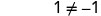
b. Is x=−1 a solution?
 |
|
| Let x = −1. | 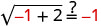 |
| Simplify. | 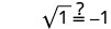 |
 |
|
| −1 is not a solution. | |
| −1 is an extraneous solution to the equation. |
For the equation \(\sqrt{x+6}=x\):
- Is x=−2 a solution?
- Is x=3 a solution?
- Answer
-
- no
- yes
Now we will see how to solve a radical equation. Our strategy is based on the relation between taking a square root and squaring.
For\(a \ge 0\), \((\sqrt{a})^2=a\)
How to Solve Radical Equations
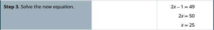
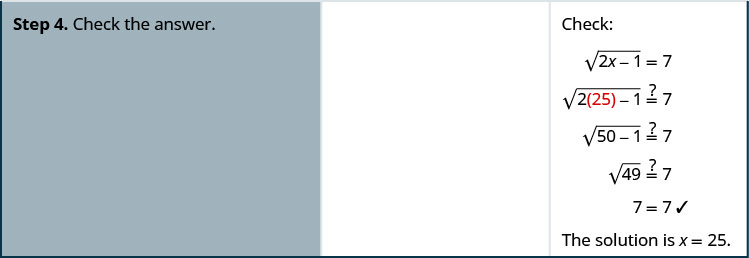
Solve: \(\sqrt{2x−1}=7\)
Solution


Solve: \(\sqrt{3x−5}=5\).
- Answer
-
10
- Isolate the radical on one side of the equation.
- Square both sides of the equation.
- Solve the new equation.
- Check the answer.
Solve: \(\sqrt{5n−4}−9=0\).
Solution
 |
|
| To isolate the radical, add 9 to both sides. | 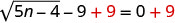 |
| Simplify. |  |
| Square both sides of the equation. | 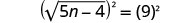 |
| Solve the new equation. |  |
 |
|
 |
|
|
Check the answer.
|
|
| The solution is n = 17. |
Solve: \(\sqrt{3m+2}−5=0\).
- Answer
-
\(\frac{23}{3}\)
Solve: \(\sqrt{3y+5}+2=5\).
Solution
 |
|
| To isolate the radical, subtract 2 from both sides. | 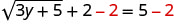 |
| Simplify. |  |
| Square both sides of the equation. |  |
| Solve the new equation. |  |
 |
|
 |
|
|
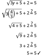
Check the answer.
|
|
| The solution is \(y=\frac{4}{3}\) |
Solve: \(\sqrt{5q+1}+4=6\).
- Answer
-
\(\frac{3}{5}\)
When we use a radical sign, we mean the principal or positive root. If an equation has a square root equal to a negative number, that equation will have no solution.
Solve: \(\sqrt{9k−2}+1=0\).
Solution
 |
|
| To isolate the radical, subtract 1 from both sides. | 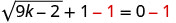 |
| Simplify. |  |
| Since the square root is equal to a negative number, the equation has no solution. |
Solve: \(\sqrt{2r−3}+5=0\)
- Answer
-
no solution
When there is a coefficient in front of the radical, we must square it, too.
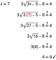
Solve: \(3\sqrt{3x−5}−8=4\).
Solution
| \(3\sqrt{3x−5}−8=4\) | |
| Isolate the radical. | \(3\sqrt{3x−5}=12\) |
| Square both sides of the equation. | \((3\sqrt{3x−5})^2=(12)^2\) |
| Simplify, then solve the new equation. | 9(3x−5)=144 |
| Distribute. | 27x−45=144 |
| Solve the equation. | 27x=189 |
| x=7 | |
|
Check the answer.
|
The solution is x=7. |
Solve: \(2\sqrt{9a+3}+14=15\).
- Answer
-
\(-\frac{11}{36}\)
Solve: \(\sqrt{4z−3}=\sqrt{3z+2}\).
Solution
| \(\sqrt{4z−3}=\sqrt{3z+2}\) | |
| The radical terms are isolated | \(\sqrt{4z−3}=\sqrt{3z+2}\) |
| Square both sides of the equation. | \((\sqrt{4z−3})^2=(\sqrt{3z+2})^2\) |
| Simplify, then solve the new equation | 4z−3=3z+2 |
| z−3=2 | |
| z=5 | |
|
Check the answer. We leave it to you to show that 5 checks! |
The solution is z=5. |
Solve: \(\sqrt{2x−5}=\sqrt{5x+3}\).
- Answer
-
\(x=\tfrac{-8}{3}\)
Use Square Roots in Applications
As you progress through your college courses, you’ll encounter formulas that include square roots in many disciplines. We have already used formulas to solve geometry applications.
We will use our Problem-Solving Strategy for Geometry Applications, with slight modifications, to develop a plan for solving applications involving formulas from any discipline.
- Read the problem carefully and ensure that all the words and ideas are understood. When appropriate, draw a figure and label it with the given information.
- Identify what we are looking for.
- Name what we are looking for by choosing a variable to represent it.
- Translate into an equation by writing the appropriate formula or model for the situation. Substitute in the given information.
- Solve the equation using good algebra techniques.
- Check the answer in the problem and make sure it makes sense.
- Answer the question with a complete sentence.
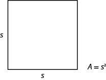
We used the formula A=L·W to find the area of a rectangle with length L and width W. A square is a rectangle in which the length and width are equal. If we let s be the length of a side of a square, the area of the square is \(s^2\).
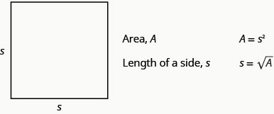
The formula \(A=s^2\) gives us the area of a square if we know the length of a side. What if we want to find the length of a side for a given area? Then we need to solve the equation for s.
\[\begin{array}{ll} {}&{A=s^2}\\ {\text{Take the square root of both sides.}}&{\sqrt{A}=\sqrt{s^2}}\\ {\text{Simplify.}}&{s=\sqrt{A}}\\ \nonumber \end{array}\]
We can use the formula \(s=\sqrt{A}\) to find the length of a side of a square for a given area.
We will illustrate this concept in the next example.
Mike and Lychelle want to make a square patio. They have enough concrete to pave an area of 200 square feet. Use the formula \(s=\sqrt{A}\) to find the length of each side of the patio. Round your answer to the nearest tenth of a foot.
Solution
| Step 1. Read the problem. Draw a figure and label it with the given information. |
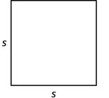 |
| A = 200 square feet | |
| Step 2. Identify what you are looking for. | The length of a side of the square patio. |
| Step 3. Name what you are looking for by choosing a variable to represent it. |
Let s = the length of a side. |
| Step 4. Translate into an equation by writing the appropriate formula or model for the situation. Substitute the given information. |
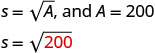 |
| Step 5. Solve the equation using good algebra techniques. Round to one decimal place. |
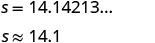 |
| Step 6. Check the answer in the problem and make sure it makes sense. |
|
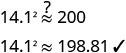 |
|
| This is close enough because we rounded the square root. Is a patio with a side of 14.1 feet reasonable? Yes. |
|
| Step 7. Answer the question with a complete sentence. |
Each side of the patio should be 14.1 feet. |
Katie wants to plant a square lawn in her front yard. She has enough sod to cover an area of 370 square feet. Use the formula \(s=\sqrt{A}\) to find the length of each side of her lawn. Round your answer to the nearest tenth of a foot.
- Answer
-
19.2 feet
Another application of square roots involves gravity.
On Earth, if an object is dropped from a height of hh feet, the time in seconds it will take to reach the ground is found by using the formula,
\(t=\frac{\sqrt{h}}{4}\)
For example, if an object is dropped from a height of 64 feet, we can find the time it takes to reach the ground by substituting h=64 into the formula.
 |
|
 |
|
| Take the square root of 64. |  |
| Simplify the fraction. |  |
It would take 2 seconds for an object dropped from a height of 64 feet to reach the ground.
Christy dropped her sunglasses from a bridge 400 feet above a river. Use the formula \(t=\frac{\sqrt{h}}{4}\) to find how many seconds it took for the sunglasses to reach the river.
Solution
| Step 1. Read the problem. | |
| Step 2. Identify what you are looking for. | The time it takes for the sunglasses to reach the river. |
| Step 3. Name what you are looking for by choosing a variable to represent it. |
Let t = time. |
| Step 4. Translate into an equation by writing the appropriate formula or model for the situation. Substitute in the given information. |
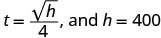 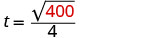 |
| Step 5. Solve the equation using good algebra techniques. |
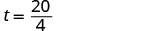  |
| Step 6. Check the answer in the problem and make sure it makes sense. |
|
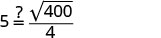 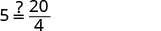 5=5✓ |
|
| Does 5 seconds seem reasonable? Yes. |
|
| Step 7. Answer the question with a complete sentence. |
It will take 5 seconds for the sunglasses to hit the water. |
A helicopter dropped a rescue package from a height of 1,296 feet. Use the formula \(t=\frac{\sqrt{h}}{4}\) to find how many seconds it took for the package to reach the ground.
- Answer
-
9 seconds
Police officers investigating car accidents measure the length of the skid marks on the pavement. Then they use square roots to determine the speed, in miles per hour, a car was going before applying the brakes.
If the length of the skid marks is d feet, then the speed, s, of the car before the brakes were applied can be found by using the formula,
\(s=\sqrt{24d}\)
After a car accident, the skid marks for one car measured 190 feet. Use the formula \(s=\sqrt{24d}\) to find the speed of the car before the brakes were applied. Round your answer to the nearest tenth.
Solution
| Step 1. Read the problem. | |
| Step 2. Identify what we are looking for. | The speed of a car. |
| Step 3. Name what we are looking for. | Let s = the speed. |
| Step 4. Translate into an equation by writing the appropriate formula. |  |
| Substitute the given information. |  |
| Step 5. Solve the equation. |  |
 |
|
| Round to 1 decimal place. |  |
| Step 6. Check the answer in the problem. 67.5≈?24(190)‾‾‾‾‾‾‾‾√ 67.5≈?4560‾‾‾‾‾√ 67.5≈?67.5277... |
|
| Is 67.5 mph a reasonable speed? | Yes. |
| Step 7. Answer the question with a complete sentence. | The car's speed was approximately 67.5 miles per hour. |
An accident investigator measured the skid marks of the car. The length of the skid marks was 76 feet. Use the formula \(s=\sqrt{24d}\) to find the speed of the car before the brakes were applied. Round your answer to the nearest tenth.
- Answer
-
42.7 mph