Section 3.3: Intercepts
- Page ID
- 188503

\( \newcommand{\vecs}[1]{\overset { \scriptstyle \rightharpoonup} {\mathbf{#1}} } \)
\( \newcommand{\vecd}[1]{\overset{-\!-\!\rightharpoonup}{\vphantom{a}\smash {#1}}} \)
\( \newcommand{\dsum}{\displaystyle\sum\limits} \)
\( \newcommand{\dint}{\displaystyle\int\limits} \)
\( \newcommand{\dlim}{\displaystyle\lim\limits} \)
\( \newcommand{\id}{\mathrm{id}}\) \( \newcommand{\Span}{\mathrm{span}}\)
( \newcommand{\kernel}{\mathrm{null}\,}\) \( \newcommand{\range}{\mathrm{range}\,}\)
\( \newcommand{\RealPart}{\mathrm{Re}}\) \( \newcommand{\ImaginaryPart}{\mathrm{Im}}\)
\( \newcommand{\Argument}{\mathrm{Arg}}\) \( \newcommand{\norm}[1]{\| #1 \|}\)
\( \newcommand{\inner}[2]{\langle #1, #2 \rangle}\)
\( \newcommand{\Span}{\mathrm{span}}\)
\( \newcommand{\id}{\mathrm{id}}\)
\( \newcommand{\Span}{\mathrm{span}}\)
\( \newcommand{\kernel}{\mathrm{null}\,}\)
\( \newcommand{\range}{\mathrm{range}\,}\)
\( \newcommand{\RealPart}{\mathrm{Re}}\)
\( \newcommand{\ImaginaryPart}{\mathrm{Im}}\)
\( \newcommand{\Argument}{\mathrm{Arg}}\)
\( \newcommand{\norm}[1]{\| #1 \|}\)
\( \newcommand{\inner}[2]{\langle #1, #2 \rangle}\)
\( \newcommand{\Span}{\mathrm{span}}\) \( \newcommand{\AA}{\unicode[.8,0]{x212B}}\)
\( \newcommand{\vectorA}[1]{\vec{#1}} % arrow\)
\( \newcommand{\vectorAt}[1]{\vec{\text{#1}}} % arrow\)
\( \newcommand{\vectorB}[1]{\overset { \scriptstyle \rightharpoonup} {\mathbf{#1}} } \)
\( \newcommand{\vectorC}[1]{\textbf{#1}} \)
\( \newcommand{\vectorD}[1]{\overrightarrow{#1}} \)
\( \newcommand{\vectorDt}[1]{\overrightarrow{\text{#1}}} \)
\( \newcommand{\vectE}[1]{\overset{-\!-\!\rightharpoonup}{\vphantom{a}\smash{\mathbf {#1}}}} \)
\( \newcommand{\vecs}[1]{\overset { \scriptstyle \rightharpoonup} {\mathbf{#1}} } \)
\(\newcommand{\longvect}{\overrightarrow}\)
\( \newcommand{\vecd}[1]{\overset{-\!-\!\rightharpoonup}{\vphantom{a}\smash {#1}}} \)
\(\newcommand{\avec}{\mathbf a}\) \(\newcommand{\bvec}{\mathbf b}\) \(\newcommand{\cvec}{\mathbf c}\) \(\newcommand{\dvec}{\mathbf d}\) \(\newcommand{\dtil}{\widetilde{\mathbf d}}\) \(\newcommand{\evec}{\mathbf e}\) \(\newcommand{\fvec}{\mathbf f}\) \(\newcommand{\nvec}{\mathbf n}\) \(\newcommand{\pvec}{\mathbf p}\) \(\newcommand{\qvec}{\mathbf q}\) \(\newcommand{\svec}{\mathbf s}\) \(\newcommand{\tvec}{\mathbf t}\) \(\newcommand{\uvec}{\mathbf u}\) \(\newcommand{\vvec}{\mathbf v}\) \(\newcommand{\wvec}{\mathbf w}\) \(\newcommand{\xvec}{\mathbf x}\) \(\newcommand{\yvec}{\mathbf y}\) \(\newcommand{\zvec}{\mathbf z}\) \(\newcommand{\rvec}{\mathbf r}\) \(\newcommand{\mvec}{\mathbf m}\) \(\newcommand{\zerovec}{\mathbf 0}\) \(\newcommand{\onevec}{\mathbf 1}\) \(\newcommand{\real}{\mathbb R}\) \(\newcommand{\twovec}[2]{\left[\begin{array}{r}#1 \\ #2 \end{array}\right]}\) \(\newcommand{\ctwovec}[2]{\left[\begin{array}{c}#1 \\ #2 \end{array}\right]}\) \(\newcommand{\threevec}[3]{\left[\begin{array}{r}#1 \\ #2 \\ #3 \end{array}\right]}\) \(\newcommand{\cthreevec}[3]{\left[\begin{array}{c}#1 \\ #2 \\ #3 \end{array}\right]}\) \(\newcommand{\fourvec}[4]{\left[\begin{array}{r}#1 \\ #2 \\ #3 \\ #4 \end{array}\right]}\) \(\newcommand{\cfourvec}[4]{\left[\begin{array}{c}#1 \\ #2 \\ #3 \\ #4 \end{array}\right]}\) \(\newcommand{\fivevec}[5]{\left[\begin{array}{r}#1 \\ #2 \\ #3 \\ #4 \\ #5 \\ \end{array}\right]}\) \(\newcommand{\cfivevec}[5]{\left[\begin{array}{c}#1 \\ #2 \\ #3 \\ #4 \\ #5 \\ \end{array}\right]}\) \(\newcommand{\mattwo}[4]{\left[\begin{array}{rr}#1 \amp #2 \\ #3 \amp #4 \\ \end{array}\right]}\) \(\newcommand{\laspan}[1]{\text{Span}\{#1\}}\) \(\newcommand{\bcal}{\cal B}\) \(\newcommand{\ccal}{\cal C}\) \(\newcommand{\scal}{\cal S}\) \(\newcommand{\wcal}{\cal W}\) \(\newcommand{\ecal}{\cal E}\) \(\newcommand{\coords}[2]{\left\{#1\right\}_{#2}}\) \(\newcommand{\gray}[1]{\color{gray}{#1}}\) \(\newcommand{\lgray}[1]{\color{lightgray}{#1}}\) \(\newcommand{\rank}{\operatorname{rank}}\) \(\newcommand{\row}{\text{Row}}\) \(\newcommand{\col}{\text{Col}}\) \(\renewcommand{\row}{\text{Row}}\) \(\newcommand{\nul}{\text{Nul}}\) \(\newcommand{\var}{\text{Var}}\) \(\newcommand{\corr}{\text{corr}}\) \(\newcommand{\len}[1]{\left|#1\right|}\) \(\newcommand{\bbar}{\overline{\bvec}}\) \(\newcommand{\bhat}{\widehat{\bvec}}\) \(\newcommand{\bperp}{\bvec^\perp}\) \(\newcommand{\xhat}{\widehat{\xvec}}\) \(\newcommand{\vhat}{\widehat{\vvec}}\) \(\newcommand{\uhat}{\widehat{\uvec}}\) \(\newcommand{\what}{\widehat{\wvec}}\) \(\newcommand{\Sighat}{\widehat{\Sigma}}\) \(\newcommand{\lt}{<}\) \(\newcommand{\gt}{>}\) \(\newcommand{\amp}{&}\) \(\definecolor{fillinmathshade}{gray}{0.9}\)We will rely heavily on these skills throughout this section.
- Identify the \(y\)-coordinate in the point \((3,5)\)
- Solve \(y=2x-1\) for \(x\) when \(y=0\)
- Solve \(y-2x=3\) for \(y\) when \(x=0\)
Motivating Problem
A heat wave is coming so you set up a lemonade stand outside the Wacheno Welcome Center. You’ve spent $10 on supplies so far, and you’re charging $0.50 per cup of lemonade. How many cups of lemonade do you need to sell before you break even (earn back the money you have put into the lemonade stand)?
Fun Fact
French mathematician Pierre de Fermat used x- and y-intercepts to study curves long before graphing calculators existed. His ideas helped pave the way for analytic geometry and modern calculus—and today, intercepts still play a key role in forecasting profits, analyzing data, and engineering designs.
The Goal
In this section, we won’t guess where lines cross the axes—we’ll learn how to find those key points directly from equations or graphs. We’ll use x- and y-intercepts as shortcuts for graphing lines and as tools to better understand how linear relationships behave.
Identify the \(x\)- and \(y\)-Intercepts on a Graph
Every linear equation can be represented by a unique line that shows all the solutions of the equation. We have seen that when graphing a line by plotting points, you can use any three solutions to graph. This means that two people graphing the line might use different sets of three points.
At first glance, their two lines might not appear to be the same, since they would have different points labeled. But if all the work was done correctly, the lines should be exactly the same. One way to recognize that they are indeed the same line is to look at where the line crosses the \(x\)-axis and the \(y\)-axis. These points are called the intercepts of the line.
The points where a line crosses the \(x\)-axis and the \(y\)-axis are called the intercepts of a line.
Let’s look at the graphs of the lines provided in the figure.
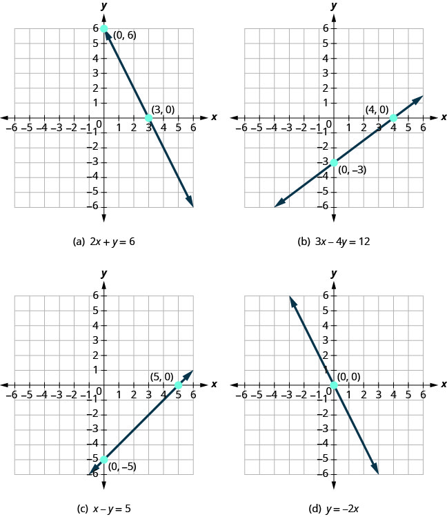
First, notice where each of these lines crosses the \(x\)-axis.
| figure | The line crosses the \(x\)-axis at: | Ordered pair of this point |
|---|---|---|
| figure (a) | 3 | (3,0) |
| figure (b) | 4 | (4,0) |
| figure (c) | 5 | (5,0) |
| figure (d) | 0 | (0,0) |
Do you see a pattern?
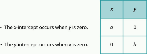
For each row, the y-coordinate of the point where the line crosses the \(x\)-axis is zero. The point where the line crosses the \(x\)-axis has the form \((a,0)\) and is called the \(x\)-intercept of a line. The \(x\)-intercept occurs when \(y\) is zero. Let’s look at the points where these lines cross the \(y\)-axis.
| figure | The line crosses the \(x\)-axis at: | Ordered pair of this point |
|---|---|---|
| figure (a) | 6 | (0,6) |
| figure (b) | −3 | (0,−3) |
| figure (c) | −5 | (0,5) |
| figure (d) | 0 | (0,0) |
What is the pattern here?
In each row, the \(x\)-coordinate of the point where the line crosses the \(y\)-axis is zero. This point has the form \((0,b)\) and is called the \(y\)-intercept of the line. The \(y\)-intercept occurs when x is zero.
The \(x\)-intercept is the point \((a,0)\) where the line crosses the \(x\)-axis.
The \(y\)-intercept is the point \((0,b)\) where the line crosses the \(y\)-axis.
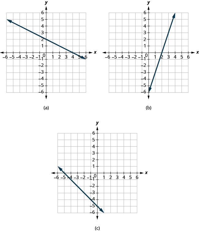
Find the \(x\)- and \(y\)-intercepts on each graph.
Solution
(a) The graph crosses the \(x\)-axis at the point \((4,0)\). The \(x\)-intercept is \((4,0)\).
The graph crosses the \(y\)-axis at the point \((0,2)\). The \(y\)-intercept is \((0,2)\).
(b) The graph crosses the \(x\)-axis at the point \((2,0)\). The \(x\)-intercept is \((2,0)\)
The graph crosses the \(y\)-axis at the point \((0,−6)\). The y- intercept is \((0,−6)\).
(c) The graph crosses the \(x\)-axis at the point \((−5,0)\). The \(x\)-intercept is \((−5,0)\).
The graph crosses the \(y\)-axis at the point \((0,−5)\). The \(y\)-intercept is \((0,−5)\).
Find the \(x\)- and \(y\)-intercepts on the graphs.
a. 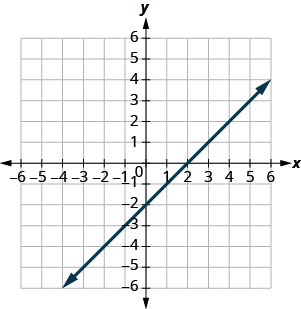 b.
b. 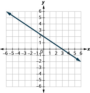
- Answer
-
a. \(x\)-intercept: \((2,0)\); \(y\)-intercept: \((0,−2)\)
b. \(x\)-intercept: \((3,0)\), \(y\)-intercept: \((0,2)\)
Find the \(x\)- and \(y\)-Intercepts from an Equation of a Line
Recognizing that the \(x\)-intercept occurs when y is zero and that the \(y\)-intercept occurs when \(x\) is zero gives us a method to find the intercepts of a line from its equation. To find the \(x\)-intercept, let \(y=0\) and solve for \(x\). To find the \(y\)-intercept, let \(x=0\) and solve for \(y\).
Use the equation of the line. To find:
- the \(x\)-intercept of the line, let \(y=0\) and solve for \(x\).
- the \(y\)-intercept of the line, let \(x=0\) and solve for \(y\).
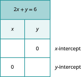
Find the intercepts of \(2x+y=6\).
Solution
We will let \(y=0\) to find the \(x\)-intercept, and let \(x=0\) to find the \(y\)-intercept. We will fill in the table, which reminds us of what we need to find.
-
To find the \(x\)-intercept, let \(y=0\).

Let \(y=0\). 
Simplify. 

The \(x\)-intercept is (3, 0) To find the \(y\)-intercept, let x = 0. 
Let x = 0. 
Simplify. 

The \(y\)-intercept is (0, 6) - The intercepts are the points \((3,0)\) and \((0,6)\).
a. Find the intercepts of \(3x+y=12\).
b. Find the intercepts of \(x+4y=8\).
- Answer
-
a. \(x\)-intercept: \((4,0)\), \(y\)-intercept: \((0,12)\)
b. \(x\)-intercept: \((8,0)\), \(y\)-intercept: \((0,2)\)
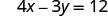
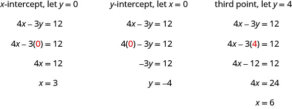
Find the intercepts of \(4x-3y=12\).
Solution
| To find the \(x\)-intercept, let y = 0. | |
 |
|
| Let y = 0. |  |
| Simplify. |  |
 |
|
 |
|
| The \(x\)-intercept is | (3, 0) |
| To find the \(y\)-intercept, let x = 0. | |
 |
|
| Let x = 0. |  |
| Simplify. |  |
 |
|
 |
|
| The \(y\)-intercept is | (0, −4) |
-
The intercepts are the points \((3, 0)\) and \((0, −4)\).
a. Find the intercepts of \(3x-4y=12\).
b. Find the intercepts of \(2x-4y=8\).
- Answer
-
a. \(x\)-intercept: \((4,0)\), \(y\)-intercept: \((0,−3)\)
b. \(x\)-intercept: \((4,0)\), \(y\)-intercept: \((0,−2)\)
Graph a Line Using the Intercepts
To graph a linear equation by plotting points, you need to find three points whose coordinates are solutions to the equation. You can use the \(x\)- and \(y\)-intercepts as two of your three points. Find the intercepts, and then find a third point to ensure accuracy. Make sure the points line up—then draw the line. This method is often the quickest way to graph a line.
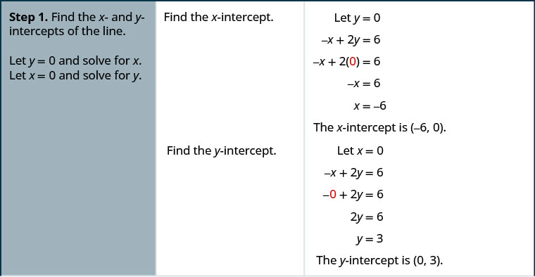
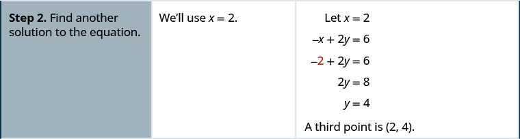
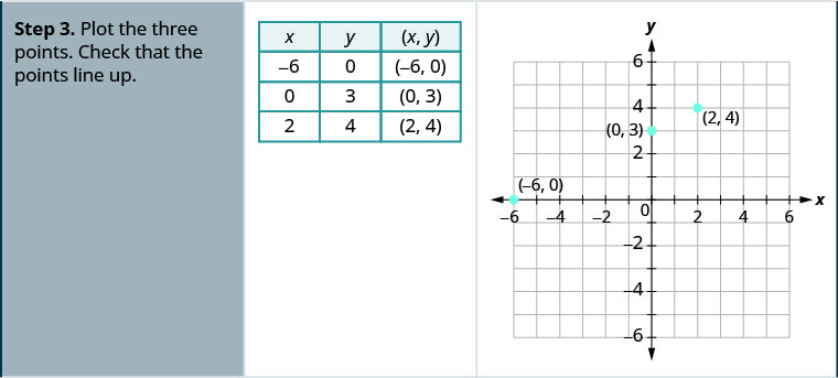
Graph \(-x+2y=6\) using the intercepts.
Solution
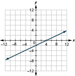
Graph \(x-2y=4\) using the intercepts.
- Answer
-
The steps to graph a linear equation using the intercepts are summarized below.
- Find the \(x\)- and \(y\)-intercepts of the line.
- Let \(y=0\) and solve for \(x\).
- Let \(x=0\) and solve for \(y\).
- Find a third solution to the equation.
- Plot the three points and check that they line up.
- Use a straight edge to draw a line through the three points.
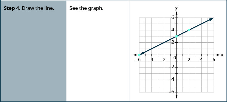
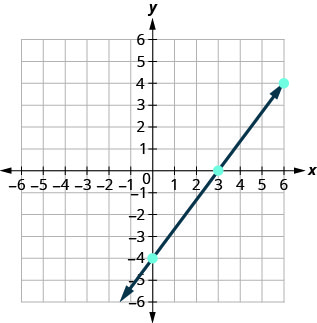
Graph \(4x-3y=12\) using the intercepts.
Solution
Find the intercepts and a third point.
We list the points in this table and show the graph below.
| \(4x−3y=12\) | ||
| \(x\) | \(y\) | \((x,y)\) |
| 3 | 0 | (3,0) |
| 0 | −4 | (0,−4) |
| 6 | 4 | (6,4) |
Graph \(5x-2y=10\) using the intercepts.
- Answer
-
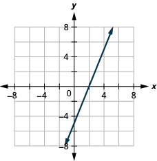
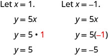
Graph \(y=5x\) using the intercepts.
Solution
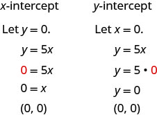
This line has only one intercept. It is the point \((0,0)\).
To ensure accuracy we need to plot three points. Since the \(x\)- and \(y\)-intercepts are the same point, we need two more points to graph the line.
| \(y=5x\) | ||
| \(x\) | \(y\) | \((x,y)\) |
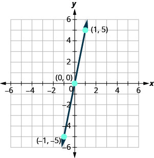
| 0 | 0 | (0,0) |
| 1 | 5 | (1,5) |
| −1 | −5 | (−1,−5) |
-
Plot the three points, check that they line up, and draw the line.
Graph \(y=−x\) using the intercepts.
- Answer
-