
1.2: Rates of Change
- Page ID
- 99692
\( \newcommand{\vecs}[1]{\overset { \scriptstyle \rightharpoonup} {\mathbf{#1}} } \)
\( \newcommand{\vecd}[1]{\overset{-\!-\!\rightharpoonup}{\vphantom{a}\smash {#1}}} \)
\( \newcommand{\dsum}{\displaystyle\sum\limits} \)
\( \newcommand{\dint}{\displaystyle\int\limits} \)
\( \newcommand{\dlim}{\displaystyle\lim\limits} \)
\( \newcommand{\id}{\mathrm{id}}\) \( \newcommand{\Span}{\mathrm{span}}\)
( \newcommand{\kernel}{\mathrm{null}\,}\) \( \newcommand{\range}{\mathrm{range}\,}\)
\( \newcommand{\RealPart}{\mathrm{Re}}\) \( \newcommand{\ImaginaryPart}{\mathrm{Im}}\)
\( \newcommand{\Argument}{\mathrm{Arg}}\) \( \newcommand{\norm}[1]{\| #1 \|}\)
\( \newcommand{\inner}[2]{\langle #1, #2 \rangle}\)
\( \newcommand{\Span}{\mathrm{span}}\)
\( \newcommand{\id}{\mathrm{id}}\)
\( \newcommand{\Span}{\mathrm{span}}\)
\( \newcommand{\kernel}{\mathrm{null}\,}\)
\( \newcommand{\range}{\mathrm{range}\,}\)
\( \newcommand{\RealPart}{\mathrm{Re}}\)
\( \newcommand{\ImaginaryPart}{\mathrm{Im}}\)
\( \newcommand{\Argument}{\mathrm{Arg}}\)
\( \newcommand{\norm}[1]{\| #1 \|}\)
\( \newcommand{\inner}[2]{\langle #1, #2 \rangle}\)
\( \newcommand{\Span}{\mathrm{span}}\) \( \newcommand{\AA}{\unicode[.8,0]{x212B}}\)
\( \newcommand{\vectorA}[1]{\vec{#1}} % arrow\)
\( \newcommand{\vectorAt}[1]{\vec{\text{#1}}} % arrow\)
\( \newcommand{\vectorB}[1]{\overset { \scriptstyle \rightharpoonup} {\mathbf{#1}} } \)
\( \newcommand{\vectorC}[1]{\textbf{#1}} \)
\( \newcommand{\vectorD}[1]{\overrightarrow{#1}} \)
\( \newcommand{\vectorDt}[1]{\overrightarrow{\text{#1}}} \)
\( \newcommand{\vectE}[1]{\overset{-\!-\!\rightharpoonup}{\vphantom{a}\smash{\mathbf {#1}}}} \)
\( \newcommand{\vecs}[1]{\overset { \scriptstyle \rightharpoonup} {\mathbf{#1}} } \)
\(\newcommand{\longvect}{\overrightarrow}\)
\( \newcommand{\vecd}[1]{\overset{-\!-\!\rightharpoonup}{\vphantom{a}\smash {#1}}} \)
\(\newcommand{\avec}{\mathbf a}\) \(\newcommand{\bvec}{\mathbf b}\) \(\newcommand{\cvec}{\mathbf c}\) \(\newcommand{\dvec}{\mathbf d}\) \(\newcommand{\dtil}{\widetilde{\mathbf d}}\) \(\newcommand{\evec}{\mathbf e}\) \(\newcommand{\fvec}{\mathbf f}\) \(\newcommand{\nvec}{\mathbf n}\) \(\newcommand{\pvec}{\mathbf p}\) \(\newcommand{\qvec}{\mathbf q}\) \(\newcommand{\svec}{\mathbf s}\) \(\newcommand{\tvec}{\mathbf t}\) \(\newcommand{\uvec}{\mathbf u}\) \(\newcommand{\vvec}{\mathbf v}\) \(\newcommand{\wvec}{\mathbf w}\) \(\newcommand{\xvec}{\mathbf x}\) \(\newcommand{\yvec}{\mathbf y}\) \(\newcommand{\zvec}{\mathbf z}\) \(\newcommand{\rvec}{\mathbf r}\) \(\newcommand{\mvec}{\mathbf m}\) \(\newcommand{\zerovec}{\mathbf 0}\) \(\newcommand{\onevec}{\mathbf 1}\) \(\newcommand{\real}{\mathbb R}\) \(\newcommand{\twovec}[2]{\left[\begin{array}{r}#1 \\ #2 \end{array}\right]}\) \(\newcommand{\ctwovec}[2]{\left[\begin{array}{c}#1 \\ #2 \end{array}\right]}\) \(\newcommand{\threevec}[3]{\left[\begin{array}{r}#1 \\ #2 \\ #3 \end{array}\right]}\) \(\newcommand{\cthreevec}[3]{\left[\begin{array}{c}#1 \\ #2 \\ #3 \end{array}\right]}\) \(\newcommand{\fourvec}[4]{\left[\begin{array}{r}#1 \\ #2 \\ #3 \\ #4 \end{array}\right]}\) \(\newcommand{\cfourvec}[4]{\left[\begin{array}{c}#1 \\ #2 \\ #3 \\ #4 \end{array}\right]}\) \(\newcommand{\fivevec}[5]{\left[\begin{array}{r}#1 \\ #2 \\ #3 \\ #4 \\ #5 \\ \end{array}\right]}\) \(\newcommand{\cfivevec}[5]{\left[\begin{array}{c}#1 \\ #2 \\ #3 \\ #4 \\ #5 \\ \end{array}\right]}\) \(\newcommand{\mattwo}[4]{\left[\begin{array}{rr}#1 \amp #2 \\ #3 \amp #4 \\ \end{array}\right]}\) \(\newcommand{\laspan}[1]{\text{Span}\{#1\}}\) \(\newcommand{\bcal}{\cal B}\) \(\newcommand{\ccal}{\cal C}\) \(\newcommand{\scal}{\cal S}\) \(\newcommand{\wcal}{\cal W}\) \(\newcommand{\ecal}{\cal E}\) \(\newcommand{\coords}[2]{\left\{#1\right\}_{#2}}\) \(\newcommand{\gray}[1]{\color{gray}{#1}}\) \(\newcommand{\lgray}[1]{\color{lightgray}{#1}}\) \(\newcommand{\rank}{\operatorname{rank}}\) \(\newcommand{\row}{\text{Row}}\) \(\newcommand{\col}{\text{Col}}\) \(\renewcommand{\row}{\text{Row}}\) \(\newcommand{\nul}{\text{Nul}}\) \(\newcommand{\var}{\text{Var}}\) \(\newcommand{\corr}{\text{corr}}\) \(\newcommand{\len}[1]{\left|#1\right|}\) \(\newcommand{\bbar}{\overline{\bvec}}\) \(\newcommand{\bhat}{\widehat{\bvec}}\) \(\newcommand{\bperp}{\bvec^\perp}\) \(\newcommand{\xhat}{\widehat{\xvec}}\) \(\newcommand{\vhat}{\widehat{\vvec}}\) \(\newcommand{\uhat}{\widehat{\uvec}}\) \(\newcommand{\what}{\widehat{\wvec}}\) \(\newcommand{\Sighat}{\widehat{\Sigma}}\) \(\newcommand{\lt}{<}\) \(\newcommand{\gt}{>}\) \(\newcommand{\amp}{&}\) \(\definecolor{fillinmathshade}{gray}{0.9}\)Focus: Describing How Quantities are Changing
If I traveled 15 miles by foot, are you impressed how fast I went? Ultimately, it depends on how long it took, the change in time. If I went 15 miles in 3 days or 72 hours, I didn't go very fast. I may have been outpaced by a tortoise. If I went 15 miles in 3 hours, that is a decent speed but not breaking any world records. In order to effectively describe the change in distance, we need to compare it to the change in another quantity such as the change in time to give it context. We write the rate of change as a ratio (or fraction) of the changes in the two quantities. \[ \dfrac{ \text{change in distance}}{ \text{change in time}} =\dfrac{15 \text{ miles}}{3 \text{ hours}} =\dfrac{5 \text{ mi.}}{1 \text{ hr.}}\nonumber \] We can simplify this fraction to find an equivalent rate of change. Traveling 15 miles in 3 hours is equivalent to traveling 5 miles per hour for three hours.
If my annual salary increased by $10,000, are you impressed? It depends. If my annual salary increased by $10,000 over the course of my adult lifetime (about 50 - 60 years), my salary hasn't increased that much considering inflation. If my annual salary increased by $10,000 over two years, that is a good raise for many people. In order to effectively describe the change in annual salary, we need to compare it to the change in another quantity such as the change in time in order to give it context. We write the rate of change as a ratio (or fraction) of the change in annual salary to the change in time. \[ \dfrac{ \text{change in annual salary}}{ \text{change in time}} =\dfrac{$10,000 }{2 \text{ years}} =\dfrac{$5,000 }{1 \text{ yr.}}\nonumber \] We can simplify this fraction to find an equivalent rate of change. An increase in annual salary of $10,000 over two years is equivalent to an increase of $5,000 per year over two years.
Key Point: Rate of Change
A rate of change is a ratio that compares the change in one quantity, such as \(y\), relative to the change in another quantity, such as \(x\). The rate of change of change is written as \[\text{rate of change} = \dfrac{ \text{change in output}}{ \text{change in input}} =\dfrac{\text{change in y}}{\text{change in x}} =\dfrac{ \Delta y} {\Delta x}\nonumber \]
We use the symbol "\( \Delta\)" to indicate the change in a quantity. For example, to indicate the change in y, we write "\( \Delta y\)". This makes writing a rate of change much simpler.
In the first introductory example, if we let \(d\) represent the change in distance and \(t\) represent the change in time, then we could write the rate of change as \[\dfrac{ \Delta d} {\Delta t} =\dfrac{5 \text{ miles}}{ 1\text{ hour}}\nonumber \]
In the second introductory example, if we let \(s\) represent the change in annual salary and \(t\) represent the change in time, then we could write the rate of change as \[\dfrac{ \Delta s} {\Delta t} =\dfrac{$5,000}{ 1\text{ year}}\nonumber \]
The rate of change we calculated in the first introductory example was not the rate of change at any one instant in the three hours I was traveling by foot. I could have started faster than 3 miles per hour, then slowed down to a rate slower than 3 miles per hour for the latter portion. I could have traveled at a constant rate of 3 miles per hour. I could have started slower than 3 miles per hour, then went faster than 3 miles per hour for the latter portion. The rate of change we calculated represents the average rate of change of distance relative to time over the three hours we traveled. The rate of change represents the rate we would travel if we traveled at a constant rate of 3 miles per hour for the whole interval.
A medication causes a patient's heart rate to increase by 20 bpm (beats per minute) when an additional 5 mg of the medication is given. Find the average rate of change in heart rate relative to amount of medication taken.
Solution
- Let \(h\) represent the change in heart rate and \(m\) represent the amount of medication. Then the average rate of change in heart rate relative to amount of medication taken can be written as \[ \dfrac{ \Delta h} {\Delta m} =\dfrac{ \text{change in heart rate}}{ \text{change in medication dosage}} =\dfrac{20 \text{ bpm}}{5 \text{ mg}} =\dfrac{4 \text{ bpm}}{1 \text{ mg}}\nonumber \] The patient's heart rate is increasing by 4 bpm per mg on average.
Some other examples of rates of change would be quantities like:
- A population of deer increases by 400 deer per year, \(\dfrac{ \Delta D} {\Delta t} = \dfrac{400 \text{ deer}}{1 \text{ year}} \).
- A barista earns $9 per hour, \( \dfrac{ \Delta M} {\Delta t} = \dfrac{$9}{1 \text{ hour}} \).
- A farmer plants 60,000 onions per acre, \( \dfrac{ \Delta O} {\Delta a} = \dfrac{60,000 \text{ onions}}{1 \text{ acre}} \).
- A car can drive 27 miles per gallon, \(\dfrac{ \Delta m} {\Delta g} = \dfrac{27 \text{ miles}}{1 \text{ gallon}} \).
- A population of grey whales decreases by 8 whales per year, \(\dfrac{ \Delta W} {\Delta t} = \dfrac{-8 \text{ whales}}{1 \text{ year}} \).
- The amount of money in your college account decreases by $4,000 per quarter, \(\dfrac{ \Delta m} {\Delta q} \dfrac{-$4,000}{1 \text{ year}} \).
Focus: Calculating Rates of Change From Data
In many cases, it may be simpler to measure data from two related quantities (or we may be given data) as opposed to measuring the changes in those two related quantities. Let's explore this situation in the following example.
Example \(\PageIndex{2}\)
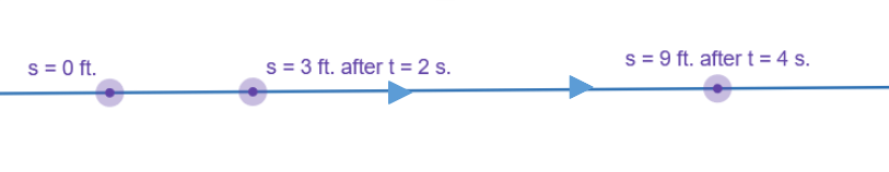
Let \(s\) represent the position of an object moving along a horizontal line after \(t\) seconds. The object was at a position of 3 feet after 2 seconts and 9 feet after 4 seconds. Find the average rate of change in position over time.
Solution
The average rate of change in position over time \[ \dfrac{ \text{change in position}}{ \text{change in time}} =\dfrac{ \Delta s}{\Delta t} = \dfrac{ s_{end} - s_{start}}{t_{end} - t_{start}} = \dfrac{9 - 3}{4 - 2} =\dfrac{6 \text{ ft.}}{2 \text{ s.}} = \dfrac{3 \text{ ft.}}{1 \text{ s.}}\nonumber \] The object's position is changing at an average rate of 3 ft. per second from \(t = 2\) s to \(t = 4\) s.
Notice in this example that we were not given the change in position. Instead, we were given the starting position and ending position. We calculated the change in position by subtracting the ending and starting position. \[ \Delta s = s_{end} - s_{start} \nonumber \]
Key Point: Average Rate of Change
The average rate of change is the ratio of the change in the output \(y\) relative to the change in the input \(x\).
\[\text{Average rate of change} = \dfrac{\text{Change of Output}}{\text{Change of Input}} = \dfrac{\Delta y}{\Delta x} =\dfrac{y_{end} -y_{start} }{x_{end} -x_{start} } \nonumber\]
The value \(V\) of a car after \(t\) years is given in the table below.
| t, years | 0 | 4 | 6 |
|---|---|---|---|
| V, Value (in US dollars) | $40,000 | $24,000 | $19,000 |
- Find the average rate of change in value from year 0 to year 4. Interpret the meaning of the rate of change in this application.
- Find the average rate of change in value over the interval [4,6]. Interpret the meaning of the rate of change in this application.
- What do the two rates of change tell you about the decrease in value of the car over time? Would you expect the rate of decrease in value to be bigger or smaller in size over the interval [6,8]?
Solution
- \[\text{Average rate of change} = \dfrac{\Delta V}{\Delta t} =\dfrac{V_{end} - V_{start} }{t_{end} -t_{start} } = \dfrac{24,000 - 40,000}{4 - 0} =\dfrac{-$16,000}{4 \text{ yr.}} = \dfrac{-$4,000}{1 \text{ yr.}}\nonumber\] The value of the car is decreasing at an average rate of $4,000 per year from year 0 to year 4.
- \[\text{Average rate of change} = \dfrac{\Delta V}{\Delta t} =\dfrac{V_{end} - V_{start} }{t_{end} -t_{start} } = \dfrac{19,000 - 24,000}{6 - 4} =\dfrac{-$5,000}{2 \text{ yr.}} = \dfrac{-$2,500}{1 \text{ yr.}}\nonumber\] The value of the car is decreasing at an average rate of $2,500 per year from year 4 to year 6.
- The rate of decrease in value over time is getting smaller in size over time. On the interval [6,8], the rate of decrease should be smaller in size (or magnitude) than $2,500 per year, such as a decrease of $2,000 per year.
When we have successive intervals of data, such as we did in the previous example, we can find the rate of change on each interval and determine what is happening to the rate of change. Determining whether the rate of increase or decrease is getting bigger or smaller in size (or magnitude) is critical in painting an even clearer and broader picture of the relationship between the two quantities we are working with.
Notice that in the last example the change of output was negative since the output value of the function had decreased. Correspondingly, the average rate of change is negative.
Now You Try: Exercise \(\PageIndex{1}\)
The number of students at Clovis Community College \(S\) during the academic year \(t\) beginning in the fall semester is given in the table below
| t, academic year | 2012 (Fall 2012-Spring 2013) | 2014 (Fall 2014-2015) | 2016 (Fall 2016-2017) |
|---|---|---|---|
| S, number of students | 7,691 | 9,020 | 10,464 |
(Unduplicated Student Enrollment as reported by The Clovis Community College Institutional Research Department)
- Find the average rate of change in the number of students at Clovis Community College from 2012 to 2014. Interpret the meaning of the rate of change in this application.
- Find the average rate of change in the number of students at Clovis Community College from 2014 to 2016. Interpret the meaning of the rate of change in this application.
- What do the two rates of change tell you about the increase in the number of students over time? Would you expect the rate of increase in the number of students to to be bigger or smaller in size from 2016 to 2018 based on this data?
- Answer
-
- The number of students is increasing at an average rate of 665 students per year from 2012 to 2014.
- The number of students is increasing at an average rate of 722 students per year from 2014 to 2016.
- The rate of increase in the number of students over time is increasing over time. From 2016-2018, the rate of increase in the number of students should be larger 722 students per year if this trend continued. An increase of 800 students per year would be reasonable based on this data.
Focus: Calculating Rates of Change with Functions
In some cases, we may be given a formula for a function. We would want to calculate the average rate of change on various intervals with the formula in order to describing a relationship with a function.
Example \(\PageIndex{4}\)
A ball is dropped from a high building. The distance in feet the ball has dropped after \(t\) seconds is given by the function \(D(t)=16t^2\), assuming negligible wind resistance.
- Find the average rate of change in the distance over time from \(t=1\) second to \(t=2\) second.
- Find the average rate of change in the distance over time over the interval [2,3].
- What is happening to the average rate of change in distance over time? Confirm your conclusion by finding the average rate of change in the distance over time over the interval [3,4].
Solution
- The average rate of change in distance over time on [1,2] \[ \dfrac{\Delta D}{\Delta t} =\dfrac{D_{end} - D_{start} }{t_{end} -t_{start} } = \dfrac{D(2)-D(1)}{2 -1 } \nonumber\] Since we are given a formula for the distance, we can evaluate the distance at our ending time \(t = 2\) to find the ending distance \(D(2)\). Similarly, we can evaulate \(D(1)\) to find our starting distance. \[\dfrac{\Delta D}{\Delta t}=\dfrac{16(2)^2 - 16(1)^2}{2 - 1} =\dfrac{64 - 16}{2 - 1} =\dfrac{48 \text{ ft}}{1 \text{ s}} \nonumber\] The ball is dropping at an average rate of 48 ft. per second from \(t=1\) seconds to \(t=2\) seconds. Note that the average rate of change of distance over time gives us the average speed on the interval.
- The average rate of change in distance over time on [2,3]\[ \dfrac{\Delta D}{\Delta t} =\dfrac{D_{end} - D_{start} }{t_{end} -t_{start} } = \dfrac{D(3)-D(2)}{3 -2 } \nonumber\] As we did in part (a), we can find the ending and starting distances \(D(3)\) and \(D(2)\), by evaluating the distance at our ending time \(t=3\) and starting time \(t=2\).\[\dfrac{\Delta D}{\Delta t}=\dfrac{16(3)^2 - 16(2)^2}{3 - 2} =\dfrac{144 - 64}{3 - 2} =\dfrac{80 \text{ ft}}{1 \text{ s}} \nonumber\] The ball is dropping at an average rate of 80 ft. per second from \(t=2\) seconds to \(t=3\) seconds.
- The average rate of change in distance over time is increasing. Effectively, ball is speeding up as it drops. The speed should be larger that \(\dfrac{80 \text{ ft}}{1 \text{ s}}\) the interval [3,4] . Calculating the average speed on the interval [3,4] \[ \dfrac{\Delta D}{\Delta t} =\dfrac{D_{end} - D_{start} }{t_{end} -t_{start} } = \dfrac{D(4)-D(3)}{4 -3 } \nonumber\] \[=\dfrac{16(4)^2 - 16(3)^2}{4 - 3} =\dfrac{256 - 144}{4 - 3} =\dfrac{112 \text{ ft}}{1 \text{ s}} \nonumber\] The ball is dropping at an average rate of 112 ft. per second from \(t=3\) seconds to \(t=4\) seconds confirming our conclusion.
We did many repetitive calculations in the last example. Moving forward, we would want to find the rate of change on many successive intervals to describe a relationship between two quantities. To make this process simpler, we can develop a formula for the average rate of change from a starting time \(t_{start}=a\) to and ending time \(t_{end}=x\). If we do this for the formula in example 1.2.4, we have \[\text{Average rate of change} = \dfrac{\Delta D}{\Delta t} =\dfrac{D_{end} - D_{start} }{t_{end} -t_{start} } = \dfrac{D(x)-D(a)}{x -a } = \dfrac{16x^2-16a^2}{x -a } \nonumber\] Factoring in the numerator \[\dfrac{\Delta D}{\Delta t}=\dfrac{16(x^2-a^2)}{x -a } = \dfrac{16(x-a)(x+a)}{x -a }\nonumber\] Then simplifying, we have a simple formula for the average rate of change in distance over time. \[\dfrac{\Delta D}{\Delta t}=16(x + a ) \nonumber\] Notice how much simpler it is to calculate the average rate of change on a specific interval in the following example than in example 1.2.4.
Example \(\PageIndex{5}\)
Use the formula for the average rate of change in distance over time for the ball in example 1.2.4 to calculate the average rate of change on the intervals
- [1,2]
- [2,3]
- [3,4]
Solution
- On the interval [1,2], our starting time \(t_{start}=a=1\) and our ending time \(t_{end}=x=2\). Using our formula for the average rate of change, we have \[\dfrac{\Delta D}{\Delta t}=16(x + a ) = 16(2+1) = 48\nonumber\]
- On the interval [2,3], our starting time \(t_{start}=a=2\) and our ending time \(t_{end}=x=3\). Using our formula for the average rate of change, we have \[\dfrac{\Delta D}{\Delta t}=16(x + a ) = 16(3+2) = 80\nonumber\]
- On the interval [3,4], our starting time \(t_{start}=a=3\) and our ending time \(t_{end}=x=4\). Using our formula for the average rate of change, we have \[\dfrac{\Delta D}{\Delta t}=16(x + a ) = 16(4+3) = 112\nonumber\]
In general, for a function \(y=f(t)\) we can develop a formula for the average rate of change from a starting value of \(t_{start}=a\) and our ending value \(t_{end}=x\) in a similar manner. \[\text{Average rate of change} = \dfrac{\Delta y}{\Delta t} =\dfrac{y_{end} - y_{start} }{t_{end} -t_{start} } = \dfrac{f(x)-f(a)}{x -a} \nonumber\] This formula for the average rate of change on the interval \([a,x]\) is called the difference quotient.
For a function \(f(t)\), the difference quotient \[\dfrac{\Delta y}{\Delta t} =\dfrac{f(x)-f(a)}{x-a} \nonumber\] is a formula for the average rate of change of f relative to t on the interval [a, x].
If we let \(h\) represent the change in t, \(\Delta t\), then the ending value of t can be represented by \(t_{end}=x=a+h\) because if we start at \(t_{start}=a\) and increase by \(h= \Delta t\) we end at \(t_{end}=x=a+h\). The ending value of y can be represented as \(y_{end}=f(a+h)\). Therefore, we can represent the formula for the the average rate of change on the interval \([a,x]\) in a second form \[\text{Average rate of change} = \dfrac{\Delta y}{\Delta t} =\dfrac{y_{end} - y_{start} }{h} = \dfrac{f(a+h)-f(a)}{h } \nonumber\].
For a function \(f(t)\), the second form of the difference quotient \[\dfrac{\Delta y}{\Delta t} =\dfrac{f(a+h)-f(a)}{h} \nonumber\] is another formula for the average rate of change of f relative to t on the interval [a, b] where \(h=\Delta t\).
There are advantages and disadvantages to each form of the difference quotient as we will see in the following examples. The first form \(\dfrac{\Delta y}{\Delta t} = \dfrac{f(x)-f(a)}{x -a} \) is somewhat simpler to evaluate. The second form \(\dfrac{\Delta y}{\Delta t} = \dfrac{f(a+h)-f(a)}{h }\) is easier to simplify since we only need to factor out a common factor of h in the numerator.
Example \(\PageIndex{6}\)
Suppose that the quantity of a product sold \(q\) when a price \(p\) is charged is given by the function \(q = f(p)=100-2p\).
- Evaluate and simplify the difference quotient \(\dfrac{\Delta q}{\Delta p} = \dfrac{f(x)-f(a)}{x -a} \) to find a formula for the average rate of change in quantity sold relative to the price on the interval [a,x].
- Use the difference quotient to find the average rate of change in quantity sold relative to the price on the interval [2.00,2.10]. What does the difference quotient tell you about the rate of change of the quantity sold relative to the price?
Solution
- The average rate of change in quantity sold relative to the price \[\dfrac{\Delta q}{\Delta p} = \dfrac{f(x)-f(a)}{x -a}= \dfrac{(100-2x)-(100-2a)}{x -a} \nonumber\] Subtracting in the numerator \[\dfrac{\Delta q}{\Delta p} = \dfrac{-2x+2a}{x -a} \nonumber\] Factoring a common factor of -2 and simplifying \[\dfrac{\Delta q}{\Delta p} = \dfrac{-2(x-a)}{x -a} = \dfrac{-2 \text{ units}}{$1 } \nonumber\]
- For any interval [a,x], the average rate of change is always \(\dfrac{-2 \text{ units}}{$1}\). The rate of change in quantity sold is decreasing at a constant rate of 2 units per $1 increase in price.
Example \(\PageIndex{7}\)
Given the function \(y=f(t) = t^2+3\)
- Evaluate and simplify the first form of the difference quotient \(\dfrac{\Delta q}{\Delta p} = \dfrac{f(x)-f(a)}{x -a} \) to find a formula for the average rate of change on the interval [a,x].
- Use the formula in part (a) to find the average rate of change on the interval [2,5].
- Use the formula in part (a) to find the average rate of change on the interval [5,9].
- Evaluate and simplify the second form of the difference quotient \(\dfrac{\Delta q}{\Delta p} = \dfrac{f(a+h)-f(a)}{h} \) to find a formula for the average rate of change on the interval [a,x] where \(h=\Delta t\)
- Use the formula in part (d) to find the average rate of change on the interval [2,5].
Solution
- The average rate of change \[\dfrac{\Delta y}{\Delta t} = \dfrac{f(x)-f(a)}{x -a} = \dfrac{(x^2+3)-(a^2+3)}{x -a} \nonumber\] Subtracting in the numerator \[\dfrac{\Delta y}{\Delta t} = \dfrac{x^2-a^2}{x -a} \nonumber\] Then factoring in the numerator and simplifying \[\dfrac{\Delta y}{\Delta t} = \dfrac{(x+a)(x-a)}{x -a} = x + a \nonumber\]
- On the interval [2,5], the starting value is \(t_{start}= a = 2\) and ending value \(t_{end}= x = 5\). Using our formula, the average rate of change is \[\dfrac{\Delta y}{\Delta t} = x + a = 5 + 2 = 7 \nonumber\]
- On the interval [5,9], the starting value is \(t_{start}= a = 5\) and ending value \(t_{end}= x = 9\). Using our formula, the average rate of change is \[\dfrac{\Delta y}{\Delta t} = x + a = 9 + 5 = 14 \nonumber\]
- The average rate of change \[\dfrac{\Delta y}{\Delta t} = \dfrac{f(a+h)-f(a)}{h} = \dfrac{((a+h)^2+3)-(a^2+3)}{h} \nonumber\] Squaring \(a+h\) and distributing the minus sign in the numerator \[\dfrac{\Delta y}{\Delta t} = \dfrac{a^2 + 2ah +h^2+3 - a^2 -3}{h} \nonumber\] Simplifying in the numerator by collecting like terms \[\dfrac{\Delta y}{\Delta t} = \dfrac{2ah +h^2}{h} \nonumber\] Factoring our a common factor of h in the numerator and simplifying, we have \[\dfrac{\Delta y}{\Delta t} = \dfrac{h(2a +h)}{h} = 2a + h\nonumber\]
- On the interval [2,5], the starting value is \(t_{start}= a = 2\), the ending value \(t_{end}= x = 5\), and \( h=\Delta t\ = 5 - 2 = 3\). Using our formula, the average rate of change is \[\dfrac{\Delta y}{\Delta t} = 2a + h = 2(2)+3 = 5 \nonumber\] Notice that the average rate of change on this interval was the same using either form of the difference quotient. Although the formulas from the two forms of the difference quotient are different and in terms of different variables, they will calculate the same average rate of change on a specific interval.
Example \(\PageIndex{8}\)
A car with an initial velocity of \(20 \dfrac{m}{s}\) accelerates with a constant acceleration of \(10 \dfrac{m}{s^2}\). The distance the car has traveled after \(t\) seconds is given by \(s(t)=5t^2+20t\).
- Evaluate and simplify either form of the difference quotient to find a formula for the average rate of change on the interval [a,x].
- Use the formula in part (a) to find the average velocity on the interval [5,10].
- Use the formula in part (a) to find the average velocity on the interval [10,15].
Solution
- Using the second form of the difference quotient, the average rate of change \[\dfrac{\Delta s}{\Delta t} = \dfrac{f(a+h)-f(a)}{h} = \dfrac{(5(a+h)^2+20(a+h))-(5a^2+20a)}{h} \nonumber\] Squaring \(a+h\) and distributing in the numerator \[\dfrac{\Delta s}{\Delta t} = \dfrac{5(a^2 + 2ah +h^2) +20a + 20h - 5a^2 -20a}{h} \nonumber\] Multiplying and simplifying in the numerator by collecting like terms \[\dfrac{\Delta s}{\Delta t} = \dfrac{5a^2+10ah +5h^2+20h-5a^2}{h} \nonumber\] Simplifying further in the numerator \[\dfrac{\Delta s}{\Delta t} = \dfrac{10ah +5h^2+20h}{h} \nonumber\] Factoring our a common factor of h in the numerator and simplifying, we have\[\dfrac{\Delta s}{\Delta t} = \dfrac{h(10a+5h+20)}{h} = 10a+5h+20\nonumber\] Although it possible to use form one of the difference quotient, it is much harder to factor and simplify than the second form.
- On the interval [5,10], the starting time is \(t_{start}= a = 5\) and the change in time \( h=\Delta t\ = 10 - 5 = 5\). Using our formula, the average velocity is \[\dfrac{\Delta s}{\Delta t} = 10a+5h+20 = 10(5)+5(5)+20 = 95 \dfrac{m}{s} \nonumber\]
- On the interval [10,15], the starting time is \(t_{start}= a = 10\) and the change in time \( h=\Delta t\ = 15 - 10 = 5\). Using our formula, the average velocity is \[\dfrac{\Delta s}{\Delta t} = 10a+5h+20 = 10(10)+5(5)+20 = 145 \dfrac{m}{s} \nonumber\]
Now You Try: Exercise \(\PageIndex{2}\)
Given the functions \(y=f(t) = 4t^2 - 1\) and \(y=g(t) = 2t^2 + 3t + 1\)
- Evaluate and simplify the first form of the difference quotient \(\dfrac{\Delta y}{\Delta t} = \dfrac{f(x)-f(a)}{x -a} \) to find a formula for the average rate of change of \(f\) on the interval [a,x].
- Use the formula in part (a) to find the average rate of change on the interval [3,7].
- Evaluate and simplify the second form of the difference quotient \(\dfrac{\Delta q}{\Delta p} = \dfrac{g(a+h)-g(a)}{h} \) to find a formula for the average rate of change of \(g\) on the interval [a,x] where \(h=\Delta t\)
- Use the formula in part (c) to find the average rate of change on the interval [1,4].
- Answer
-
- The average rate of change is \(\dfrac{\Delta y}{\Delta t} = 4(x + a) \).
- On the interval [3,7], the average rate of change is \(\dfrac{\Delta y}{\Delta t} = 40 \).
- The average rate of change is \(\dfrac{\Delta y}{\Delta t} = 4a + 2h\).
- On the interval [1,4], the average rate of change is \(\dfrac{\Delta y}{\Delta t} = 7\).
Important Topics of This Section
- Rate of Change
- Average Rate of Change
- Calculating Average Rate of Change using Function Notation
- The Difference Quotient