
1.3: Describing Relationships with Linear Functions
- Page ID
- 158862
\( \newcommand{\vecs}[1]{\overset { \scriptstyle \rightharpoonup} {\mathbf{#1}} } \)
\( \newcommand{\vecd}[1]{\overset{-\!-\!\rightharpoonup}{\vphantom{a}\smash {#1}}} \)
\( \newcommand{\dsum}{\displaystyle\sum\limits} \)
\( \newcommand{\dint}{\displaystyle\int\limits} \)
\( \newcommand{\dlim}{\displaystyle\lim\limits} \)
\( \newcommand{\id}{\mathrm{id}}\) \( \newcommand{\Span}{\mathrm{span}}\)
( \newcommand{\kernel}{\mathrm{null}\,}\) \( \newcommand{\range}{\mathrm{range}\,}\)
\( \newcommand{\RealPart}{\mathrm{Re}}\) \( \newcommand{\ImaginaryPart}{\mathrm{Im}}\)
\( \newcommand{\Argument}{\mathrm{Arg}}\) \( \newcommand{\norm}[1]{\| #1 \|}\)
\( \newcommand{\inner}[2]{\langle #1, #2 \rangle}\)
\( \newcommand{\Span}{\mathrm{span}}\)
\( \newcommand{\id}{\mathrm{id}}\)
\( \newcommand{\Span}{\mathrm{span}}\)
\( \newcommand{\kernel}{\mathrm{null}\,}\)
\( \newcommand{\range}{\mathrm{range}\,}\)
\( \newcommand{\RealPart}{\mathrm{Re}}\)
\( \newcommand{\ImaginaryPart}{\mathrm{Im}}\)
\( \newcommand{\Argument}{\mathrm{Arg}}\)
\( \newcommand{\norm}[1]{\| #1 \|}\)
\( \newcommand{\inner}[2]{\langle #1, #2 \rangle}\)
\( \newcommand{\Span}{\mathrm{span}}\) \( \newcommand{\AA}{\unicode[.8,0]{x212B}}\)
\( \newcommand{\vectorA}[1]{\vec{#1}} % arrow\)
\( \newcommand{\vectorAt}[1]{\vec{\text{#1}}} % arrow\)
\( \newcommand{\vectorB}[1]{\overset { \scriptstyle \rightharpoonup} {\mathbf{#1}} } \)
\( \newcommand{\vectorC}[1]{\textbf{#1}} \)
\( \newcommand{\vectorD}[1]{\overrightarrow{#1}} \)
\( \newcommand{\vectorDt}[1]{\overrightarrow{\text{#1}}} \)
\( \newcommand{\vectE}[1]{\overset{-\!-\!\rightharpoonup}{\vphantom{a}\smash{\mathbf {#1}}}} \)
\( \newcommand{\vecs}[1]{\overset { \scriptstyle \rightharpoonup} {\mathbf{#1}} } \)
\(\newcommand{\longvect}{\overrightarrow}\)
\( \newcommand{\vecd}[1]{\overset{-\!-\!\rightharpoonup}{\vphantom{a}\smash {#1}}} \)
\(\newcommand{\avec}{\mathbf a}\) \(\newcommand{\bvec}{\mathbf b}\) \(\newcommand{\cvec}{\mathbf c}\) \(\newcommand{\dvec}{\mathbf d}\) \(\newcommand{\dtil}{\widetilde{\mathbf d}}\) \(\newcommand{\evec}{\mathbf e}\) \(\newcommand{\fvec}{\mathbf f}\) \(\newcommand{\nvec}{\mathbf n}\) \(\newcommand{\pvec}{\mathbf p}\) \(\newcommand{\qvec}{\mathbf q}\) \(\newcommand{\svec}{\mathbf s}\) \(\newcommand{\tvec}{\mathbf t}\) \(\newcommand{\uvec}{\mathbf u}\) \(\newcommand{\vvec}{\mathbf v}\) \(\newcommand{\wvec}{\mathbf w}\) \(\newcommand{\xvec}{\mathbf x}\) \(\newcommand{\yvec}{\mathbf y}\) \(\newcommand{\zvec}{\mathbf z}\) \(\newcommand{\rvec}{\mathbf r}\) \(\newcommand{\mvec}{\mathbf m}\) \(\newcommand{\zerovec}{\mathbf 0}\) \(\newcommand{\onevec}{\mathbf 1}\) \(\newcommand{\real}{\mathbb R}\) \(\newcommand{\twovec}[2]{\left[\begin{array}{r}#1 \\ #2 \end{array}\right]}\) \(\newcommand{\ctwovec}[2]{\left[\begin{array}{c}#1 \\ #2 \end{array}\right]}\) \(\newcommand{\threevec}[3]{\left[\begin{array}{r}#1 \\ #2 \\ #3 \end{array}\right]}\) \(\newcommand{\cthreevec}[3]{\left[\begin{array}{c}#1 \\ #2 \\ #3 \end{array}\right]}\) \(\newcommand{\fourvec}[4]{\left[\begin{array}{r}#1 \\ #2 \\ #3 \\ #4 \end{array}\right]}\) \(\newcommand{\cfourvec}[4]{\left[\begin{array}{c}#1 \\ #2 \\ #3 \\ #4 \end{array}\right]}\) \(\newcommand{\fivevec}[5]{\left[\begin{array}{r}#1 \\ #2 \\ #3 \\ #4 \\ #5 \\ \end{array}\right]}\) \(\newcommand{\cfivevec}[5]{\left[\begin{array}{c}#1 \\ #2 \\ #3 \\ #4 \\ #5 \\ \end{array}\right]}\) \(\newcommand{\mattwo}[4]{\left[\begin{array}{rr}#1 \amp #2 \\ #3 \amp #4 \\ \end{array}\right]}\) \(\newcommand{\laspan}[1]{\text{Span}\{#1\}}\) \(\newcommand{\bcal}{\cal B}\) \(\newcommand{\ccal}{\cal C}\) \(\newcommand{\scal}{\cal S}\) \(\newcommand{\wcal}{\cal W}\) \(\newcommand{\ecal}{\cal E}\) \(\newcommand{\coords}[2]{\left\{#1\right\}_{#2}}\) \(\newcommand{\gray}[1]{\color{gray}{#1}}\) \(\newcommand{\lgray}[1]{\color{lightgray}{#1}}\) \(\newcommand{\rank}{\operatorname{rank}}\) \(\newcommand{\row}{\text{Row}}\) \(\newcommand{\col}{\text{Col}}\) \(\renewcommand{\row}{\text{Row}}\) \(\newcommand{\nul}{\text{Nul}}\) \(\newcommand{\var}{\text{Var}}\) \(\newcommand{\corr}{\text{corr}}\) \(\newcommand{\len}[1]{\left|#1\right|}\) \(\newcommand{\bbar}{\overline{\bvec}}\) \(\newcommand{\bhat}{\widehat{\bvec}}\) \(\newcommand{\bperp}{\bvec^\perp}\) \(\newcommand{\xhat}{\widehat{\xvec}}\) \(\newcommand{\vhat}{\widehat{\vvec}}\) \(\newcommand{\uhat}{\widehat{\uvec}}\) \(\newcommand{\what}{\widehat{\wvec}}\) \(\newcommand{\Sighat}{\widehat{\Sigma}}\) \(\newcommand{\lt}{<}\) \(\newcommand{\gt}{>}\) \(\newcommand{\amp}{&}\) \(\definecolor{fillinmathshade}{gray}{0.9}\)Focus: Describing Relationships with a Constant Rate of Change
Let's explore one of the most basic relationships between quantities where the rate of change is constant. For example, suppose we have a function \(y=f(x)\) with a constant rate of change \(\dfrac{ \Delta y} {\Delta x} =\dfrac{2}{1} \) and an initial value of \(y=1\) at \(x=0\). The rate of change tells us that for each increase in the input \(x\) of 1 causes an increase in the output \(y\) of 2. Describing this relationship with a table, at
| \(x\) | 0 | 1 | 2 | 3 | 4 |
|---|---|---|---|---|---|
| \(y=f(x)\) | 1 | 3 | 5 | 7 | 9 |
Plotting each of these points we can build a graph this function.
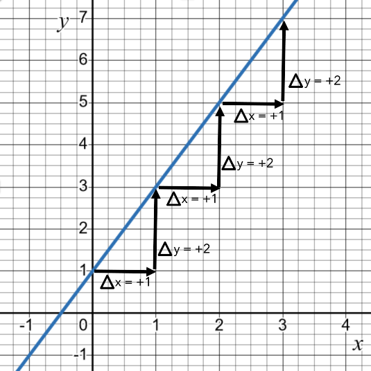
The plotting of this data reveals that the graph of this function with a constant rate of change is a line. We call a graph whose function is a line a linear function. Notice how the constant rate of change is related to the graph. Since the value of the input \(x\) is on the horizontal axis, the change in \(x\) is the horizontal change. Since the value of the output \(y\) is on the vertical axis, the change in \(y\) is the vertical change. The constant rate of change is the ratio of the vertical change to the horizontal change which graphically represents the slope or steepness of the line.\[\dfrac{ \Delta y} {\Delta x} =\dfrac{\text{change in y}}{\text{change in x}} = \dfrac{\text{vertical change}}{\text{horizontal change}} = \dfrac{\text{rise}}{\text{run}} = \text{slope m } \nonumber \] Since the rate of change is constant, the graph will rise at a constant rate for increase in \(x\) of 1 confirming that the graph is a line.
The slope of line is a ratio the vertical change to the horizontal change of the graph of the line. \[\text{slope m}= \dfrac{rise}{run} = \dfrac{\text{vertical change}}{\text{horizontal change}} = \dfrac{ \Delta y} {\Delta x} \nonumber \] The slope of a line measures the steepness of the line.
- A function with constant rate of change is a linear function whose graph is a straight line.
- The constant rate of change of a linear function is represented graphically by the slope of the line, \(m=\dfrac{ \Delta y} {\Delta x} \).
Exploring this concept further with a second function, \(y=g(x)\) with a constant rate of change \(\dfrac{ \Delta y} {\Delta x} =\dfrac{-3}{1} \) and an initial value of \(y=6\) at \(x=0\). The rate of change tells us that for each increase in our input \(x\) of 1 causes a decrease in our output \(y\) of -3. Describing this relationship with a table,
| \(x\) | 0 | 1 | 2 | 3 | 4 |
|---|---|---|---|---|---|
| \(y=g(x)\) | 6 | 3 | 0 | -3 | -6 |
Plotting each of these points we can build a graph this function.

Similarly, we see that the graph of this second function with a constant rate of change is a also line. The constant rate of change \(\dfrac{ \Delta y} {\Delta x} =\dfrac{-3}{1} = m \) describes the slope of the line confirming our conclusion. Notice that this rate of change is negative causing the line to move downward and the value of \(y\) to decrease as we move along the line from left to right since the change in \(y\) is negative. In contrast, the rate of change in the first introductory example was positive causing the line to move upward and the value of \(y\) to increase as we move along the line from left to right since the change in \(y\) is positive.
A function \(y=f(x)\) is increasing on an interval [a,b] if for any two values of \(x_{1}\) and \(x_{2}\) in the interval where \(x_{2}>x_{1} \), we have \(f(x_{2}) > f(x_{1}) \),
A function \(y=f(x)\) is decreasing on an interval [a,b] if for any two values of \(x_{1}\) and \(x_{2}\) in the interval where \(x_{2} >x_{1} \), we have \(f(x_{2}) < f(x_{1}) \),
- If a linear function \(y=f(x)\) has a positive slope \(m\), the function is increasing and the line moves upward as we move along the line from left to right.
- If a linear function \(y=f(x)\) has a negative slope \(m\), the function is decreasing and the line moves downward as we move along the line from left to right.
The temperature of the ocean off the coast of California was measured at various depths as shown in the table below (estimated results as reported by NOAA on June 7, 2024 ).
| d, depth (in feet) | 0 | 5 | 10 | 20 |
|---|---|---|---|---|
| T, Temperature (in \(^{\circ}\) F) | 60 | 58 | 56 | 52 |
Determine if the function describing the relationship between temperature and depth is linear. If so, find the slope of the line and interpret its meaning as a rate of change in the context of the application.
Solution
A function is linear if the rate of change is constant. Calculating the rate of change on each interval. On the interval [0,5], \[m = \dfrac{ \Delta T} {\Delta d} = \dfrac{58-60}{5-0} = \dfrac{-2}{5} = \dfrac{-0.4 ^{\circ} \text{F}}{1 \text{ ft}} \nonumber \] On the interval [5,10], \[m = \dfrac{ \Delta T} {\Delta d} = \dfrac{56-58}{10-5} = \dfrac{-2}{5} = \dfrac{-0.4 ^{\circ} \text{F}}{1 \text{ ft}} \nonumber \] On the interval [10,20], \[m = \dfrac{ \Delta T} {\Delta d} = \dfrac{52-56}{20-10} = \dfrac{-4}{10} = \dfrac{-0.4 ^{\circ} \text{F}}{1 \text{ ft}} \nonumber \]
The function is linear since the rate of change is constant. In the context of this application, the slope \(m = \dfrac{-0.4 ^{\circ} \text{F}}{1 \text{ ft}} \) tells us that the temperature is decreasing -0.4 \(^{\circ}\) F per foot in depth.
Although the change in Temperature is different, \( \Delta T \) = -2 versus \( \Delta T \) = -4 on the intervals [0,5] and [10,20] respectively, the rate of change is the ratio of the changes in the two quantities.
A graph of the data illustrates that the graph is a line.

The populations of two countries from 1970 - 2020 are given below (as reported by The World Bank on 6/12/24). The country of Australia experienced relatively linear growth in this time period, whereas the country of Afghanistan did not. Which country is Australia? Which country is Afghanistan?
| t, Year | 1970 | 1980 | 1990 | 2000 | 2010 | 2020 |
|---|---|---|---|---|---|---|
| Country A (in millions) | 10.75 | 12.49 | 10.69 | 19.54 | 28.19 | 38.94 |
| Country B (in millions) | 12.51 | 14.69 | 17.07 | 19.03 | 22.03 | 25.65 |
Solution
The population is linear if the rate of change is constant. Calculating the rates of change on each interval
| Time Interval | [1970,1980] | [1980,1990] | [1990,2000] | [2000,2010] | [2010,2020] |
|---|---|---|---|---|---|
| Country A, \(\dfrac{ \Delta P} {\Delta t} \) in \(\dfrac{\text{millions}} {\text{year}} \) | 0.174 | -0.18 | 0.885 | 0.865 | 1.075 |
| Country B, \(\dfrac{ \Delta P} {\Delta t} \) in \(\dfrac{\text{millions}} {\text{year}} \) | 0.218 | 0.238 | 0.196 | 0.300 | 0.362 |
Country B is experiencing the closest to linear growth since the rate of change only varies slightly from 0.196 to 0.362. The population of Country A increases for a time, then decreases, before increasing again. Therefore, Australia is Country A and Afghanistan is Country B.
The mortality rates for children under 5 years per 1,000 live births from 1995 to 2010 are given in the table below (as reported by The UN Inter-agency Group for Child Mortality Estimation on June 21, 2024)
| Year | 1995 | 2000 | 2005 | 2010 |
|---|---|---|---|---|
|
mortality rate(in \(\dfrac{\text{deaths}} {\text{yr}} \) ) |
87 | 76 | 63 | 51 |
Is the mortality rate decreasing at an approximately linear rate?
- Answer
-
Calculating the rates on change on each time interval
The rate of change in the mortality rate for children since 1995 Interval [1995,2000] [2000,2005] [2005,2010] rate of change in mortality rate per year ( in \(\dfrac{\text{deaths per year}} {\text{year}} \) ) -2.2 -2.6 -2.4 Yes, the mortality rate is decreasing at an approximately linearly. The rate of decrease in mortality rate is relatively constant varying from 2.2 \(\dfrac{\text{deaths per year}} {\text{year}} \) to 2.6 \(\dfrac{\text{deaths per year}} {\text{year}} \) and then to 2.4 \(\dfrac{\text{deaths per year}} {\text{year}} \) over this time interval .
Here is a case where the analysis we or other groups can do to effect positive change in the world by analyzing a relationship. This analysis could then helps make informed decisions on the effectiveness of programs and initiatives which could further reduce infant mortality.
Focus: More on The Slope of a Line and Rates of Change
The slope of a line measures the steepness of a line. For example, if Road A climbed 135 feet over 3900 ft and Road B climbed 120 ft. over 3175 feet at a constant steepness, which is steeper? The slopes of each road allows us to quantify and compare their steepness. The slope of Road A is \(m_{A} = \dfrac{\text{vertical change}}{\text{horizontal change}} = \dfrac{135} {3900} \approx 0.0346 \) whereas the slope of Road B is \(m_{B} = \dfrac{\text{vertical change}}{\text{horizontal change}} = \dfrac{120} {3175} \approx 0.0378 \). Road B is steeper. It climbs 0.378 feet every foot of horizontal travel whereas Road A climbs only 0.346 feet every foot of horizontal travel. Although Road A has a greater rise, it rose over a greater horizontal run making the road less steep than Road B.
Find the slope of a line containing the points (2,1) and (5,3).

Solution
The slope \( m = \dfrac{\Delta y}{\Delta x} = \dfrac{y_{end} - y_{start}}{x_{end} - x_{start}} = \dfrac{3 - 1}{5-2} = \dfrac{2} {3} \)
If we know that a function in an application has a constant rate of change, we calculate the slope in the same way from two data points in order to calculate the constant rate of change.
Suppose a company's valuation was $15 million in 2002 and rose to $80 million in 2016. Assume the company's value grew at a constant rate.
- Graph the data. Then graph a linear function relating the company's value \(V\) to the time \(t\) in years since 2000.
- Find the slope of the line.
- Interpret the slope as a rate of change in this application.
Solution
- Since we assumed that the company's value grew at a constant rate, the function is linear. The graph is given below.

- Calculating the slope \[\text{slope m}= \dfrac{\text{vertical change}}{\text{horizontal change}} = \dfrac{ \Delta V} {\Delta t} = \dfrac{80-15} {16-2} = \dfrac{65} {14} \approx $4.64 \dfrac{\text{million}} {\text{year}} \nonumber \]
- The value of the company is increasing at a constant rate of $4.64 million dollars per year.
On February 1, 2024, the discharge of the San Joaquin River out of the Millerton lake dam was 571 \(\dfrac{\text{ft}^{3}}{s} \). On April 1, 2024, the discharge was 554 \(\dfrac{\text{ft}^{3}}{s} \) (as reported by The United States Geological Survey on June 17, 2024). Assume the rate of decrease in the discharge is constant from April through May.
- Graph the data. Then graph a linear function relating the discharge \(D\) to the time \(t\) in days since February 1, 2024.
- Find the slope of the line.
- Interpret the slope as a rate of change in this application.
Solution
- Similar to the previous example, the function is linear since we assumed that the discharge decreased at a constant rate. The graph is given below.
-

- Calculating the slope \[\text{slope m}= \dfrac{\text{vertical change}}{\text{horizontal change}} = \dfrac{ \Delta D} {\Delta t} = \dfrac{554-571} {59-0} = \dfrac{-17} {59} \approx -0.288 \dfrac{\text{ft.}^{3}} {\text{day}} \nonumber \]
- The discharge out of the dam is decreasing at a rate of 0.288 \(\text{ft.}^{3}\) per day.
In applications, assuming the rate of change is constant is very big assumption and shouldn't be done lightly. In reality, more data such as that of examples 1.3.1 and 1.3.2 or some underlying physical relationship would be needed to justify such a claim. In making projections into the future for certain quantities, it is reasonable to assume the rate of change is constant as one possible projection.
Find the slope of a line containing the points (-2,3) and (3,-1).
- Answer
-
The slope \( m = \dfrac{\Delta y}{\Delta x} = \dfrac{-4} {5} \)
Suppose a medication has a side effect that causes a patient's resting heart rate to increase. With no medication, the patient's resting heart rate is 80 bpm (beats per minute). If 20 mg of the medication is taken by the patient, their resting heart rate increases to 92 bpm. Assume that the patient's heart rate increases at a constant rate.
- Graph the data. Then graph a linear function relating the patient's resting heart rate \(r\) to the dosage of the medication \(d\) in mg.
- Find the slope of the line.
- Interpret the slope as a rate of change in this application.
- Answer
-
- The function is linear since we assumed that the heart rate increased at a constant rate. The graph is given below.
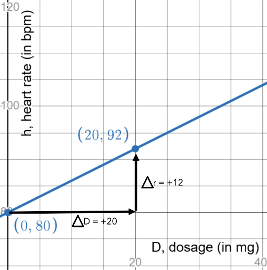
- The slope \(m = 0.6 \dfrac{\text{bpm}} {\text{mg}} \)
- The patient's resting heart rate is increasing at a rate of 0.6 bpm per mg of the medication.
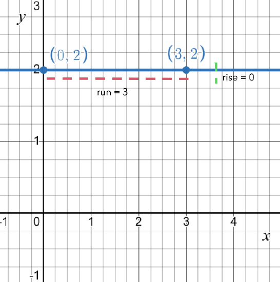
For a horizontal line, such as y = 2, the slope \(m = 0\) since the rise is zero. Calculating the slope from the points (0,2) and (3,2), the slope \( m = \dfrac{\Delta y}{\Delta x} = \dfrac{2 - 2}{3 - 0} = \dfrac{0} {3} = 0 \). Therefore, the average rate of change is zero and there is no change in \(y\).
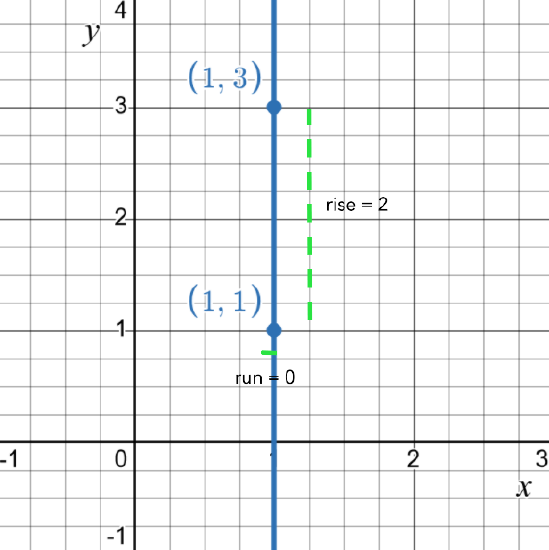
For a vertical line, such as x = 1, the slope \(m \) is undefined since the run is zero. Calculating the slope from the points (1,1) and (1,3) the slope \( m = \dfrac{\Delta y}{\Delta x} = \dfrac{3-1}{1 - 1} = \dfrac{2} {0} \). There is no change in \(x\) and so we can't compare it to the change in \(y\). Therefore, there is no rate of change that we can define.
Focus: The Formula for a Linear Function
Looking back at the introductory example of this section where we have a function \(y=f(x)\) with a constant rate of change \(\dfrac{ \Delta y} {\Delta x} =\dfrac{2}{1} \) and an initial value of \(y=1\) at \(x=0\). Notice how we can calculate each successive value of the output \(y\) with the initial value \(b = y_{0}=1\) at \(x_{0} = 0\) and the slope \(m=2\).
| x | 0 | 1 | 2 | 3 | 4 | x |
|---|---|---|---|---|---|---|
| y | 1 | 1+2(1) = 3 | 1+2(2) = 5 | 1+2(3) = 7 | 1+2(4) = 9 | 1 + 2x = y |
For any input \(x\), the output of the function can be calculated with the formula \(y = 1+ 2x\) or \(y = 2x + 1\). Notice on the graph of this function in the introductory example that the initial value \(b = y_{0}=1\) at \(x_{0} = 0\) is the y-coordinate of the y-intercept of the graph of the line. We summarize this relationship between the formula for a line and its graph with the following key point.
Key Point: The Formula for a Linear Function (Slope-Intercept Form)
The formula for a linear functions can be written in the form
\(y= f(x) = mx+b\)
where
- \(m\) is the slope of the line on the graph and the constant rate of change of the function
- \(b\) is the y-coordinate of the y-intercept on the graph and the initial value of the function at \(x\) = 0
The slope-intercept formula of a line allows us to relate the parameters of the formula to the features of the graph of the line as well as the rate of change.
Identify the slope and y-intercept of each linear function. Then graph each line.
- \(y=3x-2\)
- \(3x+4y=12\)
Solution
- Since the linear equation is in slope-intercept form as formula for y, we can identify the slope \(m = 3\) as the coefficient of x and the constant \(b = -2\) as the y-coordinate of the y-intercept. The graph is shown below left.
- Notice that this equation is not written as a formula for the output \(y\). Before we can identify the slope and y-intercept, we need to solve for \(y\). Subtracting \(3x\) from both sides \[4y = -3x + 12 \nonumber \] Then dividing both sides by 4 and simplifying \[y = \dfrac{-3} {4}y + \dfrac{12} {4} = -\dfrac{3} {4}y + 3 \nonumber \] Now that the equation is in slope-intercept form, we can identify the slope \(m = -\dfrac{3} {4}\) as the coefficient of x and the constant \(b = 3\) as the y-coordinate of the y-intercept. The graph is shown below right.


Find the equation of a line with the following properties:
- A slope \(m = 3\) that contains the point (0,5)
- A slope \(m = 3\) that contains the point (1,5)
Solution
- The point (0,5) is a y-intercept since the x-coordinate \( x = 0\) and so \(b = 5\). Using slope intercept form, the equation of the line is \( y = 3x + 5\)
- In contrast to part (a), the point here is not a y-intercept since the x-coordinate \( x \neq 0\). However, since the point \( x = 1\) and \( y = 5 \) is on the graph, it must be a solution to the equation for the line \(y=mx+b\). Substituting the known values for \( x \), \( y\), and \( m\) into the equation, we have \[5 = (3)(1) + b \nonumber \] Solving for b \[2 = b \nonumber \] Therefore, the equation of the line is \[y = 3x + 2 \nonumber \]
Alternatively, if we are given the slope \(m\) and a point \((x_{1}, y_{1})\) that is not the y-intercept of a non-vertical line, then for any other point on the line \((x, y)\) the slope of the line can be calculated as \[m = \dfrac{\Delta y} {\Delta x} = \dfrac{y - y_{1}} {x - x_{1}} \nonumber \] Multiplying both sides of the equation by \((x - x_{1})\), we have \[m(x - x_{1}) = y - y_{1} \text{ or } y - y_{1} = m(x - x_{1}) \nonumber \] This equation can be used to find the equation of a line. It is called the point-slope form of the equation of a line.
The equation of a line with slope \(m\) that contains the point \((x_{1}, y_{1})\), can be written \[y - y_{1} = m(x - x_{1}) \nonumber \]
We could have used the point-slope form of the equation of a line to solve example 1.3.7b. Substituting the slope \(m = 3\) and the point \(x_{1}=1\) and \(y_{1}=5\) into the point-slope equation of the line, we have \[y - 5 = 3 (x - 1) \nonumber \] Distributing \[y - 5 = 3 x - 3 \nonumber \] Then solving for y, we have \[y = 3 x + 2 \nonumber \]
Identify the slope and y-intercept of the linear function \( 2x - 4y = 7\). Then graph the line.
- Answer
-
Putting the equation in slope-intercept form \[y = \dfrac{1} {2}y - \dfrac{7} {4} = 0.5x - 1.75 \nonumber \] The slope \(m = \dfrac{1} {2} = 0.5\) and the y-coordinate of the y-intercept is \(b =- \dfrac{7} {4} = -1.75\).

Find the equation of a line that contains the points (1.2, 3) and (2.4,5).
- Answer
-
The slope \[m = \dfrac{\Delta y} {\Delta y} = \dfrac{5} {3} \approx 1.67 \nonumber \] Using the point-slope form of the equation of the line, \[y - 3 = 1.67(x - 1.2) \nonumber \] \[y = 1.67x +1 \nonumber \] Altervatively, we could have used the slope intercept form of the equation of a line to find the equation of the line similar to how we approached example 1.7.3b.
Focus: Modeling Relationships in Applications with Linear Functions
If we are going to use a linear function to describe a relationship between two quantities, we first need to determine if the rate of change is constant. If so, a linear function is appropriate to model the relationship. If not, we will need another type of function to describe the relationship. In order to fully describe the relationship with a linear function, we need a constant rate of change, a formula, and a graph as well as a description in words to communicate our results. Once we have a formula, we can make informed predictions about the relationship. Understanding how the formula of a linear function is related to the graph allows us to build the formula from the graph itself or information about the graph. Conversely, we can build a graph from the formula.
The average listing price of a home in Fresno, California was $363,832 in January 2017. The price increased at an average rate of $6,522 per year from 2017 to 2019 (as reported by The Federal Reserve Bank on June 26,2024). Assume the average listing price continues to increase at this rate.
- Find a formula for a linear function \(P = f(t) \) for the average listing price P in terms of t, the years since 2017. Then graph the function.
- Predict the average listing price in 2025 if the price continues to increase at this rate.
- When will the average listing price reach $400,000?
Solution
- A linear function is appropriate to model this relationship, since we are assuming the rate of change is constant. The initial data point \(t=0\), \(P = $363,832\) is a P-intercept (or y-intercept if \(y=P\)). So \(b = 363,832\). The constant rate of change $6,522 is our slope \(m\). Using the slope-intercept form of the equation of a line, the formula for this linear function is \[P = f(t) = 6,522t + 363.832 \nonumber\]
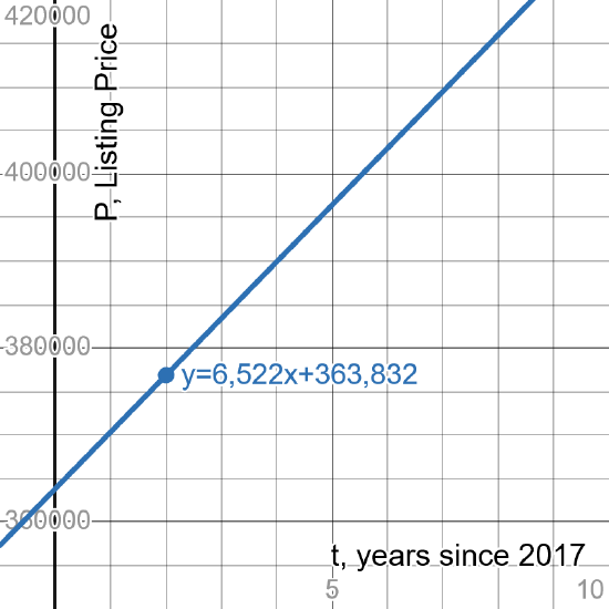
- The year 2025 is \(t = 8\) years after 2017. Using our formula for the average listing price \[P = f(8) = 6,522(8) + 363,832 = 416,008 \nonumber\] The average listing price of a home in Fresno, California in 2025 will be $416,008 according our model. If we are able to obtain additional data, we could determine the accuracy of the constant rate of change and our prediction.
- Substituting the given listing price \( P = 400,000 \) into our formula \[400,000 = 6,522t + 363,832 \nonumber\] Solving for t by subtracting 363,832 \[36,168 = 6,522t \nonumber\] Dividing by 6,522 \[t = \dfrac{36,168} {6,522} \approx 5.56 \nonumber\] The average listing price of a home in Fresno, California will reach $400,000 in mid-2022 if the price keeps increasing at constant rate.
Example \(\PageIndex{9}\)
Marcus currently owns 200 songs in his iTunes collection. Every month, he adds 15 new songs. Write a formula for the number of songs, \(N\), in his iTunes collection as a function of the number of months, \(m\). How many songs will he own in a year?
Solution
The initial value for this function is 200, since he currently owns 200 songs, so \(N(0)=200\). The number of songs increases at a constant rate of 15 songs per month which represents the slope of the line on the graph. With this information, we can write the formula:
\[N(m)=200+15m\nonumber \]
\(N(m)\) is an increasing linear function. With this formula we can predict how many songs he will have in 1 year (12 months):
\[N(12)=200+15(12)=200+180=380\nonumber \] Marcus will have 380 songs in 12 months.
Example \(\PageIndex{10}\)
The pressure, \(P\), in pounds per square inch (PSI) on a diver depends upon their depth below the water surface, \(d\), in feet, following the equation \(P(d)=14.696+0.434d\). Interpret the parameters of this function in the context of this application.
Solution
The rate of change, or slope, \(m = 0.434\) has units \(m = \dfrac{\Delta P}{\Delta d} = \dfrac{\text{PSI}}{\text{ft}}\). This tells us the pressure on the diver increases by 0.434 PSI for each foot of depth.
The initial value, 14.696, will have the same units as the output, so this tells us that at a depth of 0 feet, the pressure on the diver will be 14.696 PSI.
Example \(\PageIndex{11}\)
The cumulative percentage of adults vaccinated with the updated 2023-2024 COVID-19 vaccine was 14.7% in December 2023 and grew to 21.1% in February 2024 (as reported by The CDC vaccines on June 26,2024). Assume the percentage of adults vaccinated increases at a constant rate.
- Find a formula for a linear function \(P = f(t) \) for the cumulative percentage of adults vaccinated in terms of t, the months since December 2023.
- Interpret the slope as a rate of change.
- Predict the cumulative percentage of adults vaccinated in June 2024, if the vaccination continues to increase at this rate.
Solution
- A linear function is appropriate to model this relationship, since we are assuming the rate of change is constant. The initial data corresponds to the point \(t=0\), \(P = 14.7\) which is a P-intercept (or y-intercept if \(y=P\) ). So \(b = 14.7\). We can use the two data points, \( (t,P) = (0,14.7) \text{ and } (t,P) = (2,21.1) \) to calculate the slope of the line. \[m = \dfrac{\Delta P}{\Delta t} = \dfrac{21.1 - 14.7} {2 - 0} = \dfrac{6.4} {2} = 3.2 \nonumber\] Using the slope-intercept form of the equation of a line, the formula for this linear function is \[P = f(t) = 3.2t + 14.7 \nonumber\]
- Notice the units of the slope as a rate of change \[m = \dfrac{\Delta P}{\Delta t} = \dfrac{\text{%}}{\text{month}} \nonumber\] The slope tells us that the cumulative percentage of adults getting the updated COVID-19 vaccine is increasing at an average rate of 3.2% per month over this period.
- June 2024 corresponds to \(t = 6\) months since December 2023. Using our formula, \[P = 3.2(6) + 14.7 = 33.9 \nonumber\] The cumulative percentage of adults vaccinated with the updated 2023-2024 COVID-19 vaccine will 33.9% in June 2024 according our model. If additional data became available that showed the rate of increase began to get smaller, our prediction would be an overestimate.
In the winter of 2020, the United States was experiencing the Omicron wave of the COVID pandemic. In the week of October 3, 2020, the number of deaths in the US from COVID-19 was 4,240 per week. Nine weeks later, in the week of December 5, 2020 the number of deaths was 18,545 per week (as reported by The CDC on June 26,2024). At that point in time, no further data was available. In order to predict future weekly COVID death rates moving forward at that time, assume the number of deaths increases at a constant rate.
- Find a formula for a linear function \(D = f(t) \) for the number of deaths from COVID-19 per week in terms of t, the weeks since October, 3 2020.
- Interpret the slope as a rate of change.
- Predict the the number of weekly deaths from COVID-19 in the week of February 6, 2021, 19 weeks from October 3, 2020 if the vaccination continues to increase at this rate.
- Answer
-
- The D-intercept (or y-intercept if \(y=D\)) is \(b = 4,240\). The slope is \(m = \dfrac{\Delta D}{\Delta t} = \dfrac{14,305} {9} \approx 1,589 \). The formula for this linear function is \[D = f(t) = 1,589t + 4,240 \nonumber\]
- Notice the units of the slope as a rate of change \[m = \dfrac{\Delta D}{\Delta t} = \dfrac{\text{weekly deaths}}{\text{week}} \nonumber\] The slope tells us that the the number of deaths from COVID-19 per week was increasing at an average rate of 1,589 per week over this period.
- In 19 weeks, the number number of weekly deaths from COVID-19 in the week of February 6, 2021 was 34,431 according our model.
Although the rate of increase in deaths actually increased over this period, it eventually slowed down and the COVID deaths per week peaked during the week of January 9, 2021 at 25,924 before dropping. At that point in time, medical, governmental, business, and other organizations needed informed predictions in order to plan an effective response. The modeling we have done is a basic type of modeling that could have been used as a portion of that response.
Many relationships between two quantities do not have a rate of change that is constant as we saw in the last exercise. Moving forward, we need to explore and analyze other functions to help us describe relationships where the rate of change is not constant. This will encompass our broader goal for the entirety of the remainder of the text.
Important Topics of this Section
- Definition of a linear function
- Formula of a linear function
- Increasing & Decreasing linear functions
- Finding the y-intercept
- Finding the slope/rate of change, m
- Modeling in applications with linear functions