
2.4: Solving Exponential Equations with Logarithms
- Page ID
- 99714
\( \newcommand{\vecs}[1]{\overset { \scriptstyle \rightharpoonup} {\mathbf{#1}} } \)
\( \newcommand{\vecd}[1]{\overset{-\!-\!\rightharpoonup}{\vphantom{a}\smash {#1}}} \)
\( \newcommand{\dsum}{\displaystyle\sum\limits} \)
\( \newcommand{\dint}{\displaystyle\int\limits} \)
\( \newcommand{\dlim}{\displaystyle\lim\limits} \)
\( \newcommand{\id}{\mathrm{id}}\) \( \newcommand{\Span}{\mathrm{span}}\)
( \newcommand{\kernel}{\mathrm{null}\,}\) \( \newcommand{\range}{\mathrm{range}\,}\)
\( \newcommand{\RealPart}{\mathrm{Re}}\) \( \newcommand{\ImaginaryPart}{\mathrm{Im}}\)
\( \newcommand{\Argument}{\mathrm{Arg}}\) \( \newcommand{\norm}[1]{\| #1 \|}\)
\( \newcommand{\inner}[2]{\langle #1, #2 \rangle}\)
\( \newcommand{\Span}{\mathrm{span}}\)
\( \newcommand{\id}{\mathrm{id}}\)
\( \newcommand{\Span}{\mathrm{span}}\)
\( \newcommand{\kernel}{\mathrm{null}\,}\)
\( \newcommand{\range}{\mathrm{range}\,}\)
\( \newcommand{\RealPart}{\mathrm{Re}}\)
\( \newcommand{\ImaginaryPart}{\mathrm{Im}}\)
\( \newcommand{\Argument}{\mathrm{Arg}}\)
\( \newcommand{\norm}[1]{\| #1 \|}\)
\( \newcommand{\inner}[2]{\langle #1, #2 \rangle}\)
\( \newcommand{\Span}{\mathrm{span}}\) \( \newcommand{\AA}{\unicode[.8,0]{x212B}}\)
\( \newcommand{\vectorA}[1]{\vec{#1}} % arrow\)
\( \newcommand{\vectorAt}[1]{\vec{\text{#1}}} % arrow\)
\( \newcommand{\vectorB}[1]{\overset { \scriptstyle \rightharpoonup} {\mathbf{#1}} } \)
\( \newcommand{\vectorC}[1]{\textbf{#1}} \)
\( \newcommand{\vectorD}[1]{\overrightarrow{#1}} \)
\( \newcommand{\vectorDt}[1]{\overrightarrow{\text{#1}}} \)
\( \newcommand{\vectE}[1]{\overset{-\!-\!\rightharpoonup}{\vphantom{a}\smash{\mathbf {#1}}}} \)
\( \newcommand{\vecs}[1]{\overset { \scriptstyle \rightharpoonup} {\mathbf{#1}} } \)
\(\newcommand{\longvect}{\overrightarrow}\)
\( \newcommand{\vecd}[1]{\overset{-\!-\!\rightharpoonup}{\vphantom{a}\smash {#1}}} \)
\(\newcommand{\avec}{\mathbf a}\) \(\newcommand{\bvec}{\mathbf b}\) \(\newcommand{\cvec}{\mathbf c}\) \(\newcommand{\dvec}{\mathbf d}\) \(\newcommand{\dtil}{\widetilde{\mathbf d}}\) \(\newcommand{\evec}{\mathbf e}\) \(\newcommand{\fvec}{\mathbf f}\) \(\newcommand{\nvec}{\mathbf n}\) \(\newcommand{\pvec}{\mathbf p}\) \(\newcommand{\qvec}{\mathbf q}\) \(\newcommand{\svec}{\mathbf s}\) \(\newcommand{\tvec}{\mathbf t}\) \(\newcommand{\uvec}{\mathbf u}\) \(\newcommand{\vvec}{\mathbf v}\) \(\newcommand{\wvec}{\mathbf w}\) \(\newcommand{\xvec}{\mathbf x}\) \(\newcommand{\yvec}{\mathbf y}\) \(\newcommand{\zvec}{\mathbf z}\) \(\newcommand{\rvec}{\mathbf r}\) \(\newcommand{\mvec}{\mathbf m}\) \(\newcommand{\zerovec}{\mathbf 0}\) \(\newcommand{\onevec}{\mathbf 1}\) \(\newcommand{\real}{\mathbb R}\) \(\newcommand{\twovec}[2]{\left[\begin{array}{r}#1 \\ #2 \end{array}\right]}\) \(\newcommand{\ctwovec}[2]{\left[\begin{array}{c}#1 \\ #2 \end{array}\right]}\) \(\newcommand{\threevec}[3]{\left[\begin{array}{r}#1 \\ #2 \\ #3 \end{array}\right]}\) \(\newcommand{\cthreevec}[3]{\left[\begin{array}{c}#1 \\ #2 \\ #3 \end{array}\right]}\) \(\newcommand{\fourvec}[4]{\left[\begin{array}{r}#1 \\ #2 \\ #3 \\ #4 \end{array}\right]}\) \(\newcommand{\cfourvec}[4]{\left[\begin{array}{c}#1 \\ #2 \\ #3 \\ #4 \end{array}\right]}\) \(\newcommand{\fivevec}[5]{\left[\begin{array}{r}#1 \\ #2 \\ #3 \\ #4 \\ #5 \\ \end{array}\right]}\) \(\newcommand{\cfivevec}[5]{\left[\begin{array}{c}#1 \\ #2 \\ #3 \\ #4 \\ #5 \\ \end{array}\right]}\) \(\newcommand{\mattwo}[4]{\left[\begin{array}{rr}#1 \amp #2 \\ #3 \amp #4 \\ \end{array}\right]}\) \(\newcommand{\laspan}[1]{\text{Span}\{#1\}}\) \(\newcommand{\bcal}{\cal B}\) \(\newcommand{\ccal}{\cal C}\) \(\newcommand{\scal}{\cal S}\) \(\newcommand{\wcal}{\cal W}\) \(\newcommand{\ecal}{\cal E}\) \(\newcommand{\coords}[2]{\left\{#1\right\}_{#2}}\) \(\newcommand{\gray}[1]{\color{gray}{#1}}\) \(\newcommand{\lgray}[1]{\color{lightgray}{#1}}\) \(\newcommand{\rank}{\operatorname{rank}}\) \(\newcommand{\row}{\text{Row}}\) \(\newcommand{\col}{\text{Col}}\) \(\renewcommand{\row}{\text{Row}}\) \(\newcommand{\nul}{\text{Nul}}\) \(\newcommand{\var}{\text{Var}}\) \(\newcommand{\corr}{\text{corr}}\) \(\newcommand{\len}[1]{\left|#1\right|}\) \(\newcommand{\bbar}{\overline{\bvec}}\) \(\newcommand{\bhat}{\widehat{\bvec}}\) \(\newcommand{\bperp}{\bvec^\perp}\) \(\newcommand{\xhat}{\widehat{\xvec}}\) \(\newcommand{\vhat}{\widehat{\vvec}}\) \(\newcommand{\uhat}{\widehat{\uvec}}\) \(\newcommand{\what}{\widehat{\wvec}}\) \(\newcommand{\Sighat}{\widehat{\Sigma}}\) \(\newcommand{\lt}{<}\) \(\newcommand{\gt}{>}\) \(\newcommand{\amp}{&}\) \(\definecolor{fillinmathshade}{gray}{0.9}\)Goal: Solving Exponential Equations
In the previous section, we encountered exponential equations where the variable is in the exponent, such as
\[10=2^{x} .\nonumber\]
We can solve this equation graphically by graphing the curve \(y=2^{x}\) and the line \(y=10\) then approximating the point of intersection in the graph below.
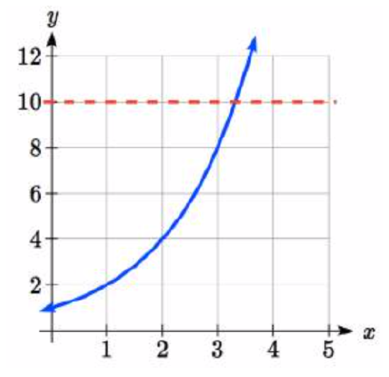
The point of intersection is approximately at \(x \approx3.3\). Therefore, the solution to the equation \(x \approx3.3\).
However, in many applications in mathematics, science, and engineering, it would be necessary to have the exact solution or at least a more accurate approximation.
Focus: Solving Exponential Equations Analytically
To solve the equation, \(10=2^{x}\), we need to find the exponent of 2. Our strategy to do this is to create a function that tells us the exponent.
Case: Base 10
The logarithm base 10 of x is the exponent of 10 that gives x. We write \(\log _{10} (x) = y\) if and only if \(10^{y}=x\).
We read \(\log _{10} (x)\) as "log base 10 of x".
The logarithm base 10 is a function whose output is the exponent of 10. In other words, the logarithm base 10 tells us the exponent of 10. Notice each logarithmic statement is equivalent to the corresponding exponential statement. Also, the inputs and outputs are switched with a logarithm and the corresponding exponential statement. Effectively, we have defined the logarithm base 10, \(f^{-1}(x) = log _{10} (x) \), as the inverse function of the exponential function base 10, \(f(x) = 10^{x}\). Let's explore this correspondence between exponential and logarithmic form and the definition of a logarithm in the following examples.
Write these exponential equations as logarithmic equations:
- \(10^{2} =100\)
- \(10^{4} =10000\)
- \(10^{-4} =\dfrac{1}{10000}\)
Solution
a) \(10^{2} =100\) is equivalent to \(\log _{10} (100)=2\)
b) \(10^{4} =10000\) is equivalent to \(\log _{10} (10000)=4\)
c) \(10^{-4} =\dfrac{1}{10000}\) is equivalent to \(\log _{10} \left(\dfrac{1}{10000} \right)=-4\)
Write these logarithmic equations as exponential equations:
a) \(\log _{10} (1000)=3\)
b) \(\log _{10} (5) \approx 0.69897\)
Solution
a) \(\log _{10} (1000)=3\) is equivalent to \(10^{3} =1000\)
b) \(\log _{10} (5) \approx 0.69897\) is equivalent to \(10^{0.69897} \approx 5\)
On a calculator, the \(log\) button calculates the \(\log _{10}\), the logarithm base 10. Try and use your calculator to calculate a decimal approximation of \(\log _{10} (5)\).
Case: Base b, where b > 1 or 0 < b < 1
The logarithm base b of x is the exponent of b that gives x. We write \(\log _{b} (x) = y\) if and only if \(b^{y}=x\).
We read \(\log _{b} (x)\) as "log base b of x".
In this case, the logarithm base b is a function whose output is the exponent of b. In other words, the logarithm base b tells us the exponent of b. Effectively, we have defined the logarithm base b, \(f^{-1}(x) = log _{b} (x) \), as the inverse function of the exponential function base b, \(f(x) = b^{x}\).There is a similar relationship between each logarithmic equation and the corresponding exponential equation. Let's further explore this correspondence in the examples below.
Write these exponential equations as logarithmic equations:
- \(2^{3} = 8\)
- \(3^{4} =81\)
- \(e^{0} =1\)
Solution
a)\(2^{3} = 8\) is equivalent to \(\log _{2} (8)=3\)
b) \(3^{4} =81\) is equivalent to \(\log _{3} (81)=4\)
c) \(e^{0} =1\) is equivalent to \(\log _{e} (1) = 0\)
Write these logarithmic equations as exponential equations:
a) \(\log _{7} (49)=2\)
b) \(\log _{5} (625) =4\)
Solution
a) \(\log _{7} (49)=2\) is equivalent to \(7^{2} = 49\)
b) \(\log _{5} (625) =4\) is equivalent to \(5^{4} = 625\)
The logarithm base e is a very important logarithmic function. We give it a special name.
The logarithm base e is also called the natural logarithm. The natural logarithm of x is the exponent of e the gives x. We write \(\ln(x) = y\) if and only if \(e^{y}=x\).
By writing, \(\ln(x) = y\) we mean \(\log _{e} (x)=y\)
Definition: logarithm base
In example 3.4.3c, we could write \(\log _{e} (1) = 0\) or \(\ln(1) = 0\). Both statements mean the same thing.
On a calculator, the \(ln\) button calculates the natural logarithm or \(\log _{e}\) of a number. For most calculators, log base 10 and the natural log are the only logarithmic functions on the calculator. At this point, we need to develop some tools in order to find decimal approximations of logarithms of other bases.
Now you try some examples converting back and forth between exponential and logarithmic form.
Write these exponential equations as logarithmic equations:
- \(6^{4} = 1296\)
- \(10^{x} =17\)
- \(e^{2} \approx 7.389\)
- Answer
-
a) \(6^{4} = 1296\) is equivalent to \(\log _{6} (1296)=4\)
b) \(10^{x} =17\) is equivalent to \(\log _{10} (17)=x\)
c) \(e^{2} \approx 7.389\) is equivalent to \(\ln(7.389) \approx 2\)
Write these logarithmic equations as exponential equations:
a) \(\log _{5} (25)=2\)
b) \(\log _{4} (x) =3\)
c) \(\ln(5) \approx 1.609\)
- Answer
-
a) \(\log _{5} (25)=2\) is equivalent to \(5^{2} = 25\)
a) \(\log _{4} (x) =3\) is equivalent to \(4^{3} = x\)
a) \(\ln(5) \approx 7.389\) is equivalent to \(e^{1.609} = 5\)
Notice, in student exercise 3.4.1b, you started with the exponential equation with the variable x in the exponent.
\[10^{x} =17\nonumber\]
By converting to logarithmic form, you have the exponent and solution to the equation.
\[x = log _{10} (17) \approx 1.23 \nonumber\]
You can use a calculator to get a decimal approximation. This highlights a way to solve exponential equations by converting them to logarithmic form.
Solve the exponential equations.
a) \(e^{x} = 12\)
b) \(5^{x} = 7\)
c) \(3(10)^{x}+1 = 11\)
d) \(2(4)^{5x}+3 = 17\)
Solution
a) To solve the equation \[e^{x} = 12\nonumber\]
convert to logarithmic form. \[\ln(12)=x\nonumber\]
Using a calculator to find a decimal approximation, we have \(x \approx 2.4849\).
b) To solve the equation \[5^{x} = 7\nonumber\]
convert to logarithmic form. \[\log _{5} (7) =x\nonumber\]
With the tools we have developed so far, we can't use a calculator to find a decimal approximation since this logarithm is not base 10 or e.
c) Notice in parts a and b, the equation has the exponential term on one side and a number on the other. In this form, we have defined the equivalent logarthimic form. In the equation \[3(10)^{x}+1 = 11\nonumber\]
the exponential term \((10)^{x}\) is not isolated on one side of the equation. First, we need to isolate the exponential term by subtracting 1.
\[3(10)^{x} = 10\nonumber\] Then dividing by 3, we have
\[(10)^{x} =\dfrac{10}{3} . \nonumber\] Now converting to logarithmic form, we have
\[x = \log _{10} (\dfrac{10}{3} ) \approx 0.5229 \nonumber\]
d) To solve the equation \[2(4)^{5x}-3 = 17 \nonumber\] we need to isolate the exponential term by adding 3.
\[2(4)^{5x} = 20 \nonumber\] Then dividing by 2, we have
\[(4)^{5x} =\dfrac{20}{2} =10. \nonumber\] Now converting to logarithmic form, we have
\[\log _{4} (10) =5x .\nonumber\] Finally, dividing both sides of the equation by 5, we have
\[\dfrac{\log _{4} (10)}{5} = x .\nonumber\]
With the tools we have currently, we can't use a calculator to find a decimal approximation since this logarithm is not base 10 or e.
Now you try to solve a few exponential equations.
Solve the exponential equations. Find a decimal approximation if possible with the tools we have up to this point.
a) \(10^{x} = 47\)
b) \(7(3)^{x} = 12\)
c) \(4(e)^{0.012x} + 1 = 15\)
- Answer
-
a) To solve the equation \[10^{x} = 47\nonumber\]
convert to logarithmic form. \[x = \log _{10} (47) \approx 1.672 \nonumber\]
b) To solve the equation \[7(3)^{x} = 12\nonumber\] we need to isolate the exponential term by dividing by 7.
\[(3)^{x} =\dfrac{12}{7} \nonumber\] Now converting to logarithmic form, we have
\[\log _{3} (\dfrac{12}{7}) = x \nonumber\] With the tools we have currently, we can't use a calculator to find a decimal approximation since this logarithm is not base 10 or e.
c) To solve the equation \[4(e)^{0.012x} + 1 = 15 , \nonumber\] first we need to isolate the exponential term by subtracting 1.
\[4(e)^{0.012x} = 14 \nonumber\] Then dividing by 4, we have
\[e^{0.012x} =\dfrac{14}{4} = \dfrac{7}{2} = 3.5. \nonumber\] Now converting to logarithmic form, we have
\[ln(3.5) = 0.012x .\nonumber\] Finally, dividing both sides of the equation by 0.012, we have
\[x = \dfrac{ln(3.5)}{0.012} \approx 104.39 .\nonumber\]
Focus: Solving Logarithmic Equations
In the students exercise 3.4.2b, you started with the logarithmic equation with the variable x inside the logarithm \[\log _{4} (x) =3 . \nonumber\]
By converting to exponential form, you get the variable out of the logarithm and ultimately the solution to the equation. \[x = 4^{3} = 64\nonumber\] This highlights a way to solve logarithmic equations by converting them to exponential form.
Solve the logarithmic equations.
a) \(\log _{3} (x) = 4 \)
b) \(3\log _{2} (4t) = 20 \)
Solution
a) To solve the equation \[\log _{3} (x) = 4 \nonumber\]
convert to exponential form. \[x= 3^{4} = 81 \nonumber\]
b) Notice in part a, the equation has the logarithmic term on one side and a number on the other. In this form, we have defined the equivalent exponential form. In the equation \[3\log _{2} (4t) = 20\nonumber\]
the logarithmic term \(\log _{2} (4t)\) is not isolated on one side of the equation. First, we need to isolate the logarithmic term by dividing by 3.
\[\log _{2} (4t) = \dfrac{20}{3} \nonumber\] Then convert to exponential form.
\[2^{\tfrac{20}{3}} = 4t \nonumber\] Finally, to isolate t we divide by 4.
\[t = \dfrac{2^{\tfrac{20}{3}} }{4} \approx 25.398 \nonumber\]
Now you try a few exercises solving logarithmic Equations
Solve the logarithmic equations.
a) \(ln(x) = 7 \)
b) \(5\log _{6} (7t)+3 = 20 \)
- Answer
-
a) To solve the equation \[\ln(x) = 7 \nonumber\]
convert to exponential form. \[x = e^{7} \approx 1096.63 \nonumber\]
b) To solve the equation \[5\log _{6} (7t)+3 = 20 \nonumber\] we need to isolate the logarithmic term.
\[5\log _{6} (7t)= 17 \nonumber\]
\[\log _{6} (7t)= \dfrac{17}{5} = 3.4 \nonumber\] Then convert to exponential form.
\[6^{3.4} = 7t \nonumber\] Finally, to isolate t we divide by 4.
\[t=\dfrac{6^{3.4}}{7} \approx 63.18 \nonumber\]
Goal: Finding a decimal approximation of logarithms of other bases than 10 or e
One issue that remains when solving exponential equations is finding a decimal approximation of logarithms of bases other than 10 or e on most calculators. Before we can do this, we need to develop some more properties of logarithms.
1) The inverse property of logarithms \[\log _{b} \left(b^{x} \right)=x\] \[b^{log _{b}(x)}=x\]
2) The power property of logarithms \[\log _{b} \left(x^{n} \right)=n\log _{b} \left(x\right)\]
For property 3.4.1, the logarithm base b by definition gives us the exponent of b. In this case, the exponent of b is x. Additional, this highlights that the logarithm function base b , \(f(x) = \log _{b}(x) \), and the exponential function base b, \(g(x) = b^{x}\) are inverses. Property 3.4.2 is an additional result of the log and exponential functions being inverses.
For property 3.4.3, we offer a proof:
Let \(k=\log _{b} (x^{n})\). Converting to exponential form, we get \(b^{k}=x^{n}\).
Solving for x by raising both sides of the equation to the \(\dfrac{1}{n}\) power , we have \(\left(b^{k} \right)^{\tfrac{1}{n}} = \left(x^{n} \right)^{\tfrac{1}{n}}\).
Using the power property of exponents, we have \(\left(b^{\tfrac{k}{n}} \right) = x^{\tfrac{n}{n}} = x\).
Now converting to logarithmic form \(\log _{b} \left(x \right)=\dfrac{k}{n}\) and solving for k, we have \(k=n\log _{b} (x)\).
Notice that k is equivalent to the expressions on both sides of the equation in property 3.4.3.
Notice that property 3.4.1 has a logarithm and exponential functions of the same base, whereas property 3.4.3 deals with logarithms and exponential functions of the different bases. Let's try a few examples to get comfortable using these properties
Rewrite the following logarithmic expressions using the properties of logarithms.
a) \(\log _{3} \left(3^7\right)\)
b) \(ln(e^{x})\)
c) \(\log _{3} \left(5^7\right)\)
d) \(ln(2^{x})\)
Solution
a) Since the logarithmic function and the exponential function have the same base, we can use the inverse property of logarithms 3.4.1. Log base 3 gives us the exponent of 3. So
\[\log _{3} \left(3^7\right) = 7\nonumber\]
b) Again, the logarithmic function and the exponential function have the same base, so we can us the inverse property of logarithms. Log base e gives us the exponent of e. So
\[ln(e^{x}) = x\nonumber\]
c) Notice, the logarithmic function and the exponential function have different bases, so we will need to use the power property of logarithms 3.4.3.
\[\log _{3} \left(5^7\right)=7\log _{3} (5) \nonumber\]
d) Again, the logarithmic function and the exponential function have different bases, so use the power property of logarithms.
\[ln(2^{x})=x\left(ln(2)\right) \nonumber\]
Evaluate the expressions using the logarithmic properties
a) \(\ln \left(\sqrt{e} \right)\).
b) \(2^{\log _{2}(3)}\)
Solution
a) We can rewrite \(\ln \left(\sqrt{e} \right)\) as \(\ln \left(e^{1/2} \right)\). Since ln is a log base \(e\), we can use the inverse property for logs: \[\ln \left(e^{1/2} \right)=\log _{e} \left(e^{1/2} \right)=\dfrac{1}{2}\nonumber\].
b) The logarithmic function and the exponential function have the same base, so the inverse property 3.4.2 applies \(2^{\log _{2}(3)}= 3\).
Notice in example 3.4.8, by using the power property of logarithms on \(ln(2^{x})=x\left(ln(2)\right) \), we get the variable out of the logarithm. Utilizing this strategy gives us an alternative way to solve an exponential equation from which we can find a decimal approximation no matter what base of logarithm.
Solve \(2^{x}=3\) in two ways
a) By taking the natural logarithm of both sides of the equation and using the power property of logarithms to solve.
b) Converting to log form.
Solution
a) Strategy #1:
Applying the ln on both sides, we have \(ln(2^{x})=ln(3)\). Then using the power property of logarithms, we have
\[x\left(ln(2)\right)=ln(3).\nonumber\] Then solving for x we have:
\[x = \dfrac{ln(3)}{ln(2)} \approx1.585\nonumber\]
b) Strategy #2: Convert to log from.
\[x=log _{2}(3)\nonumber\]
Previously, we were unable to find a decimal approximation of \(log _{2}(3)\). However, notice the approximation of x with strategy #1 is also and approximation of the logarithm expression we found using strategy #2. Notice, this gives us a way to approximate logs of any base using a calculator.
\[\log _{2} \left(3\right)=\dfrac{ln(3)}{ln(2)}\nonumber\]
We can generalize what we have done in example 3.4.9 to approximate logarithms of any base with the following property.
\[\log _{b} \left(a\right)=\dfrac{ln(a)}{\ln(b)}\nonumber\]
Let \(\log _{b} \left(a\right)=x\).
Rewriting as an exponential gives \(b^{x} =a\).
Taking the ln of both sides of this equation gives
\[ln(b^{x}) = ln(a)\nonumber\]
Now utilizing the power property for logs on the left side,
\[x ln(b) = ln(a) \nonumber\]
Dividing, we obtain \(x=\dfrac{ln(a)}{ln(b)}\). Replacing our original expression for \(x\),
\[\log _{b} (a)=\dfrac{ln(a)}{ln(b)} \nonumber\]
Notice that the change of base formula can be written with a logarithm of any base on both sides of the equation if we start by taking the logarithm base b of both sides. We have chosen the natural logarithm since it can be approximated on a standard calculator.
Evaluate using the change of base formula.
a) \(\log _{2} (10)\)
b) \(\log _{5} (100)\)
Solution
a) Writing the logarithm with natural log we have: \(\log _{2} 10=\dfrac{\ln 10}{\ln 2} \approx 3.3219\)
b) \(\log _{5} 100=\dfrac{\ln 100}{\ln 5} \approx 2.861\nonumber\)
The change of base formula highlights two ways that we can get the solution to an exponential equation like \(2^{x} =10\) and get a decimal approximation on a standard calculator.
Strategy #1
- Isolate the exponential expressions when possible
- Convert the equation to logarithm form
- Use algebra to solve for the variable.
- Use the change of base formula to find a decimal approximation if needed.
Strategy #2
- Isolate the exponential expressions when possible
- Take the natural logarithm of both sides
- Utilize the exponent property for logarithms to pull the variable out of the exponent
- Use algebra to solve for the variable.
Solve \(2^{x} =10\) for \(x\)
a) Using strategy #1
b) Using Strategy #2
Solution
a) Converting to logarithmic for:
\[\log _{2} (10)=x\nonumber\] Using the change of base formula, we have
\[x=\dfrac{\ln (10)}{ln(2)} \approx 3.3219\nonumber\]
b) Taking the natural logarithm of both sides of the equation:
\[ln \left(2^{x} \right)=ln (10)\nonumber\] Utilizing the exponent property for logs,
\[x \left(ln(2)\right)=ln (10)\nonumber\] Now dividing by ln(2),
\[x=\dfrac{\ln (10)}{ln(2)} \approx 3.3219\nonumber\]
Notice that this result matches the result we found using the change of base formula.
Solve \(5(1.07)^{3t} =2\)
a) Using strategy #1.
b) Using Strategy #2.
Solution
a) To start, we want to isolate the exponential part of the exponential expression, \((1.07)^{3t}\), on one side of the equation.
\[5(1.07)^{3t} =2\nonumber\] Divide both sides by 5 to isolate the exponential expression.
\[(1.07)^{3t} =\dfrac{2}{5} = 0.4\nonumber\] Convert to log form.
\[\log _{1.07} (0.4) = 3t\nonumber\] Solve for t by divide by 3 on both sides.
\[\left(\dfrac{\log _{1.07} (0.4)}{3} \right)\nonumber\] Now use the change of base formula to find a decimal approximation.
\[t=\dfrac{ln(0.4)}{3ln(1.07)} \approx -4.5143\nonumber\]
b) To start, we want to isolate the exponential part of the exponential expression, \((1.07)^{3t}\), on one side of the equation as we did in part a.
\[5(1.07)^{3t} =2\nonumber\] Divide both sides by 5 to isolate the exponential
\[(1.07)^{3t} =\dfrac{2}{5} = 0.4 \nonumber\] Take the ln of both sides.
\[ln((1.07)^{3t} ) = ln(0.4)\nonumber\] Use the power property for logs
\[3t \left(ln(1.07)\right) = ln(0.4)\nonumber\] Divide by \(3\left(ln(1.07)\right)\) on both sides
\[t=\dfrac{ln(0.4)}{3ln(1.07)} \approx -4.5143\nonumber\]
Evaluate \(\log _{3} (7)\) using the change of base formula.
- Answer
-
Writing the logarithm with natural log we have: \(\log _{3} 7=\dfrac{\ln 7}{\ln 3} \approx 1.7712\)
Solve \(5(0.93)^{x} =10\) using any method. Find a decimal approximation.
- Answer
-
Using Strategy 1:
\[5(0.93)^{x} =10\nonumber\] Divide both sides by 5 to isolate the exponential expression.
\[(0.93)^{x} =\dfrac{10}{5} = 2\nonumber\] Convert to log form.
\[\log _{0.93} (2) = x\nonumber\] Now use the change of base formula to find a decimal approximation.
\[t=\dfrac{ln(2)}{ln(0.93)} \approx -9.5513\nonumber\]Using Strategy 2:
\[5(0.93)^{x} =10\nonumber\] Divide both sides by 5 to isolate the exponential expression.
\[(0.93)^{x} =\dfrac{10}{5} = 2\nonumber\] Take the ln of both sides.
\[ln((0.93)^{x} ) = ln(2)\nonumber\] Use the power property for logs
\[x \left(ln(0.93)\right) = ln(2)\nonumber\] Divide by \(\left(ln(0.93)\right)\) on both sides
\[t=\dfrac{ln(2)}{ln(0.93)} \approx -9.5513\nonumber\]
Focus: More of Modeling With Exponential Functions
In section 3.3, we highlighted two issues when modeling with exponential functions. The first issue arose when making predictions where the output was known and the input was desired. Now that we can solve exponential equations with logarithms, we can make these predictions.
In sec. 3.2, we predicted the population (in billions) of India \(t\) years after 2008 by using the function \(f(t)=1.14(1.0134)^{t}\). Note that we used a periodic exponential model, since the growth factor \(b=1.0134\) =101.34% is easily found from the given percentage growth rate \(r=0.0134\)=1.34%. If the population continues following this trend, when will the population reach 2 billion?
Solution
We need to solve for time \(t\) so that \(f(t) = 2\). Using strategy #2.
\[2=1.14(1.0134)^{t}\nonumber\] Divide by 1.14 to isolate the exponential expression
\[\dfrac{2}{1.14} =1.0134^{t}\nonumber\] Take the logarithm of both sides of the equation
\[\ln \left(\dfrac{2}{1.14} \right)=\ln \left(1.0134^{t} \right)\nonumber\] Apply the exponent property on the right side
\[\ln \left(\dfrac{2}{1.14} \right)=t\ln \left(1.0134\right)\nonumber\] Divide both sides by ln(1.0134)
\[t=\dfrac{\ln \left(\dfrac{2}{1.14} \right)}{\ln \left(1.0134\right)} \approx 42.23\text{ years}\nonumber\]
If this growth rate continues, the model predicts the population of India will reach 2 billion about 42 years after 2008, or approximately in the year 2050.
The second issue arose when trying to find the continuous growth rate r of a continuous exponential model given two data points. Now that we can solve exponential equations with logarithms, we can find continuous exponential models.
A population grows from 100 to 130 in 2 weeks.
a) Find a continuous exponential model for the population P in t weeks.
b) Predict when the population will reach 200.
Solution
a) Measuring \(t\) in weeks, we are looking for an equation \(P(t)=ae^{rt}\) so that \(P(0)\) = 100 and \(P(2)\) = 130. Our initial value is \(a\) = 100.
Using other data point t = 2 and P = 130,
\[130=100e^{r\cdot 2}\nonumber\] Divide by 100
\[\dfrac{130}{100} =e^{2r}\nonumber\] Take the natural log of both sides
\[\ln (1.3)=\ln \left(e^{2r} \right)\nonumber\] Use the inverse property of logs
\[\begin{array}{l} {\ln (1.3)=2r} \\ {r=\dfrac{\ln (1.3)}{2} \approx 0.1312} \end{array}\nonumber\]
This population is growing at a continuous rate of 13.12% per week.
The population in t weeks is given by the function \(P(t)=100e^{0.1312t}\)
b) We want the time t when P = 200. Substituting this into our model. \[P(t)=100e^{0.1312t}\nonumber\] Divide by 100
\[\dfrac{200}{100} = 2 = e^{0.1312t}\nonumber\] Take the natural log of both sides
\[\ln (2)=\ln \left(e^{0.1312t} \right)\nonumber\] Use the inverse property of logs
\[\begin{array}{l} {\ln (2) = 0.1312t} \\ {t=\dfrac{\ln (2)}{0.1312} \approx 52.83} \end{array}\nonumber\]
The population will reach 200 in approximately 53 weeks.
In 1960, the \(CO_2\) emissions was measured at 316.9 ppm (parts per million) at the Mauna Loa Observatory in Hawaii. In 2000, the \(CO_2\) emissions were measured at 369.4 ppm (NOAA - Global Monitoring Laboratory at gml.noaa.gov/ccgg/trends/global.html).
a) Find a continuous exponential model for the \(CO_2\) emissions,C , in t years since 1960.
b) Predict the \(CO_2\) emissions in 2030.
Solution
a) We have two data points given. The first, \(C(0)\) = 316.9 gives us our initial value is \(a\) = 316.9.
Substituting other data point \(C(40)\) = 369.4 into our continuous exponential model, \(C(t)=ae^{rt}\), we have
\[369.4=316.9e^{r\cdot 40}\nonumber\] Divide by 316.9
\[\dfrac{369.4}{316.9} =e^{r40}\nonumber\]
\[1.16567=e^{r40}\nonumber\] Take the natural log of both sides
\[\ln (1.16567)=\ln \left(e^{r40} \right)\nonumber\] Use the inverse property of logs
\[\begin{array}{l} {\ln (1.16567)=40r} \\ {r=\dfrac{\ln (1.16567)}{40} \approx 0.0038324} \end{array}\nonumber\]
The formula for the \(CO_2\) emissions t years since 1960 is given by the function \(C(t)=316.9e^{0.0038324t}\)
b) In 2030, t = 70. Substituting this into our model. \[C(t)=316.9e^{0.0038324(70)} \approx 414.4 ppm \nonumber\]
In 2030, the \(CO_2\) emissions will be 414.4 ppm.
Newton’s Law of Cooling
When a hot object is left in surrounding air that is at a lower temperature, the object’s temperature will decrease towards the surrounding air temperature. The difference in temperature between and object and the surrounding air temperature is an exponential function. This is the basis for Newton's Law of Cooling.
The difference in temperature between an object and the surrounding air , \(D\), is described by the exponential function
\[D(t)=ae^{kt}\]
Therefore the temperature of an object, \(T\), in surrounding air with temperature \(T_{s}\) will behave according to the formula
\[T(t)=ae^{kt} +T_{s}\]
Where
- \(t\) is time
- \(a\) is a constant determined by the initial temperature of the object
- \(k\) is a constant, the continuous rate of cooling of the object
While an equation of the form \(T(t)=ab^{t} +T_{s}\) could be used, the continuous growth form is more common.
A cheesecake is taken out of the oven with an ideal internal temperature of 165 degrees Fahrenheit, and is placed into a 35 degree refrigerator. After 10 minutes, the cheesecake has cooled to 150 degrees. If you must wait until the cheesecake has cooled to 70 degrees before you eat it, how long will you have to wait?
Solution
Since the surrounding air temperature in the refrigerator is 35 degrees, the cheesecake’s temperature will decay exponentially towards 35, following the equation
\[T(t)=ae^{kt} +35\nonumber\]
We know the initial temperature was 165, so \(T(0)=165\). Substituting in these values,
\[\begin{array}{l} {165=ae^{k0} +35} \\ {165=a+35} \\ {a=130} \end{array}\nonumber\]
We were given another pair of data, \(T(10)=150\), which we can use to solve for \(k\)
\[150=130e^{k10} +35\nonumber\]
\[\begin{array}{l} {115=130e^{k10} } \\ {\dfrac{115}{130} =e^{10k} } \\ {\ln \left(\dfrac{115}{130} \right)=10k} \\ {k=\dfrac{\ln \left(\dfrac{115}{130} \right)}{10} =-0.0123} \end{array}\nonumber\]
Together this gives us the equation for cooling: \[T(t)=130e^{-0.0123t} +35\nonumber\]
Now we can solve for the time it will take for the temperature to cool to 70 degrees.
\[70=130e^{-0.0123t} +35\nonumber\]
\[35=130e^{-0.0123t}\nonumber\]
\[\dfrac{35}{130} =e^{-0.0123t}\nonumber\]
\[\ln \left(\dfrac{35}{130} \right)=-0.0123t\nonumber\]
\[t=\dfrac{\ln \left(\dfrac{35}{130} \right)}{-0.0123} \approx 106.68\nonumber\]
It will take about 107 minutes, or one hour and 47 minutes, for the cheesecake to cool. Of course, if you like your cheesecake served chilled, you’d have to wait a bit longer.
Now you try a few examples of modeling with continuous exponential functions.
Cancer cells sometimes increase in size exponentially. Suppose a cancerous growth contained 300 cells last month and 360 cells this month.
a) Find a continuous exponential model for the number off cancer cells, C, in t months.
b) Predict how long will it take for the number of cancer cells to double?
- Answer
-
a) We are given two data points: this month, (0, 360), and last month, (-1, 300). The first point gives us our initial value is \(a\) = 360.
Substituting other data point \(C(-1)\) = 300 into our continuous exponential model, \(C(t)=ae^{rt}\), we have
\[300=360e^{r\cdot -1}\nonumber\] Divide by 360
\[\dfrac{300}{360} =e^{r(-1)}\nonumber\]\[\dfrac{5}{6} =e^{r(-1)}\nonumber\] Take the natural log of both sides
\[\ln(\dfrac{5}{6})=\ln \left(e^{r(-1)} \right)\nonumber\] Use the inverse property of logs\[\begin{array}{l} {\ln (\dfrac{5}{6})=(-1)r} \\ {r=\dfrac{ln(\tfrac{5}{6})}{-1} \approx 0.18232} \end{array}\nonumber\]
The formula for the number of cancer cells in t months is given by the function \(C(t)=360e^{0.18232t}\)
b) If the number of cells double, then C = 2(360)=720. Substituting this into our model and solving for t. \[720=360e^{0.18232t} \nonumber\]
Divide by 360
\[\dfrac{720}{360} =e^{0.18232t}\nonumber\]\[2=e^{0.18232t}\nonumber\] Take the natural log of both sides
\[\ln(2)=\ln \left(e^{0.18232t} \right)\nonumber\] Use the inverse property of logs\[\begin{array}{l} {\ln(2)=0.18232t} \\ {r=\dfrac{ln(2)}{0.18232} \approx 3.802} \end{array}\nonumber\]
The value \(V\), in billions of dollars, of US imports from China in the 2000 was 100 billion. By 2004, the value rose to 196 billion
a) Find a continuous exponential model for The value \(V\), in billions of dollars, of US imports from China \(t\) years after 2000.
b) If this trend continues, predict the value of US imports to China in 2025.
- Answer
-
a) We have two data points given. The first, \(V(0)\) = 100 gives us our initial value is \(a\) = 100.
Substituting other data point \(V(4)\) = 196 into our continuous exponential model, \(V(t)=ae^{rt}\), we have
\[196=100e^{r\cdot 4}\nonumber\] Divide by 100
\[\dfrac{196}{100} =e^{r4}\nonumber\]\[1.96=e^{r4}\nonumber\] Take the natural log of both sides
\[\ln (1.96)=\ln \left(e^{r4} \right)\nonumber\] Use the inverse property of logs\[\begin{array}{l} {\ln (1.96)=4r} \\ {r=\dfrac{\ln (1.96)}{4} \approx 0.16824} \end{array}\nonumber\]
The formula for the The value \(V\), in billions of dollars, of US imports from China t years after 2000 is given by the function \(V(t)=100e^{0.16824t}\)
b) In 2025, t = 25. Substituting this into our model. \[V(t)=100e^{0.16824(25)} \approx 6708.8 \nonumber\] The value of US imports in 2025 is $6,708.8 billion = 6.7088 trillion.
A pitcher of water at 40 degrees Fahrenheit is placed into a 70 degree room. One hour later the temperature has risen to 45 degrees. How long will it take for the temperature to rise to 60 degrees?
- Answer
-
\(T(t) = ae^{kt} + 70\). Substituting (0, 40), we find \(a = -30\). Substituting (1, 45), we solve \[45 = -30 e^{k(1)} + 70\nonumber\] to get \[k = ln(\dfrac{25}{30}) = -0.1823\nonumber\]
Solving \(60 = -30e^{-0.1823t} + 70\) gives
\[t = \dfrac{ln(1/3)}{-0.1823} = 6.026\text{ hours}\nonumber \]
Important Topics of this Section
- The Logarithmic function as the inverse of the exponential function
- Writing logarithmic & exponential expressions
- Properties of logs
- Inverse properties
- Exponential properties
- Change of base
- Common log
- Natural log
- Solving exponential equations
- Newton’s law of cooling