
6.2: Continuous Probability Functions


- Last updated
- May 6, 2023
- Save as PDF
( \newcommand{\kernel}{\mathrm{null}\,}\)
We begin by defining a continuous probability density function. We use the function notation f(x). Intermediate algebra may have been your first formal introduction to functions. In the study of probability, the functions we study are special. We define the function f(x) so that the area between it and the x-axis is equal to a probability. Since the maximum probability is one, the maximum area is also one. For continuous probability distributions, PROBABILITY = AREA.
Example 6.2.1
Consider the function f(x)=120 for 0≤x≤20. x= a real number. The graph of f(x)=120 is a horizontal line. However, since 0≤x≤20, f(x) is restricted to the portion between x=0 and x=20, inclusive.
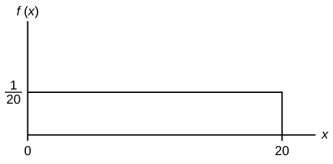 Figure 6.2.1
f(x)=120 for 0≤x≤20.
The graph of f(x)=120 is a horizontal line segment when 0≤x≤20.
The area between f(x)=120 where 0≤x≤20 and the x-axis is the area of a rectangle with base = 20 and height = 120.
AREA=20(120)=1
Suppose we want to find the area between f(x)=120 and the x-axis where 0<x<2.
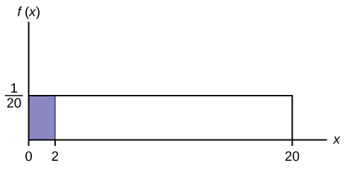 Figure 6.2.2
AREA=(2−0)(120)=0.1
(2−0)=2=base of a rectangle
REMINDER: area of a rectangle = (base)(height).
The area corresponds to a probability. The probability that x is between zero and two is 0.1, which can be written mathematically as P(0<x<2)=P(x<2)=0.1.
Suppose we want to find the area between f(x)=120 and the x-axis where 4<x<15.
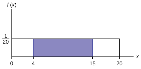 Figure 6.2.3
AREA=(15–4)(120)=0.55
AREA=(15–4)(120)=0.55
(15–4)=11=the base of a rectangle(15–4)=11=the base of a rectangle
The area corresponds to the probability P(4<x<15)=0.55.
Suppose we want to find P(x=15). On an x-y graph, x=15 is a vertical line. A vertical line has no width (or zero width). Therefore, P(x=15)=(base)(height)=(0)(120)=0
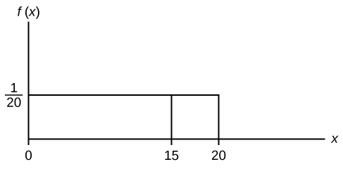 Figure 6.2.4
P(X≤x) (can be written as P(X<x) for continuous distributions) is called the cumulative distribution function or CDF. Notice the "less than or equal to" symbol. We can use the CDF to calculate P(X>x). The CDF gives "area to the left" and P(X>x) gives "area to the right." We calculate P(X>x) for continuous distributions as follows: P(X>x)=1–P(X<x).
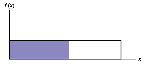 Figure 6.2.5
Label the graph with f(x) and x. Scale the x and y axes with the maximum x and y values. f(x)=120, 0≤x≤20.
To calculate the probability that x is between two values, look at the following graph. Shade the region between x=2.3 and x=12.7. Then calculate the shaded area of a rectangle.
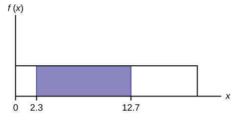 Figure 6.2.6
P(2.3<x<12.7)=(base)(height)=(12.7−2.3)(120)=0.52
Exercise 5.2.1
Consider the function f(x)=18 for 0≤x≤8. Draw the graph of f(x) and find P(2.5<x<7.5).
Answer
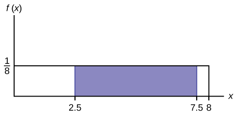 Figure 6.2.7
P(2.5<x<7.5)=0.625
Summary
The probability density function (pdf) is used to describe probabilities for continuous random variables. The area under the density curve between two points corresponds to the probability that the variable falls between those two values. In other words, the area under the density curve between points a and b is equal to P(a<x<b). The cumulative distribution function (cdf) gives the probability as an area. If X is a continuous random variable, the probability density function (pdf), f(x), is used to draw the graph of the probability distribution. The total area under the graph of f(x) is one. The area under the graph of f(x) and between values a and b gives the probability P(a<x<b).
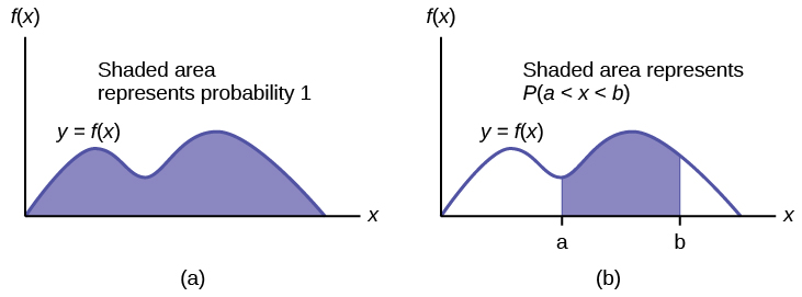 Figure 6.2.8
The cumulative distribution function (cdf) of X is defined by P(X≤x). It is a function of x that gives the probability that the random variable is less than or equal to x.
Formula Review
Probability density function (pdf) f(x):
- f(x)≥0
- The total area under the curve f(x) is one.
Cumulative distribution function (cdf): P(X≤x)
Contributors
Barbara Illowsky and Susan Dean (De Anza College) with many other contributing authors. Content produced by OpenStax College is licensed under a Creative Commons Attribution License 4.0 license. Download for free at http://cnx.org/contents/30189442-699...b91b9de@18.114.