2.6: Limits at Infinity

Learning Objectives

• Calculate the limit of a function as $x$ increases or decreases without bound.
• Recognize a horizontal asymptote on the graph of a function.

In this section, we define limits at infinity and show how these limits affect the graph of a function.

We begin by examining what it means for a function to have a finite limit at infinity. Then we study the idea of a function with an infinite limit at infinity.

Limits at Infinity and Horizontal Asymptotes

Recall that $\displaystyle \lim_{x→a}f(x)=L$ means $f(x)$ becomes arbitrarily close to $L$ as long as $x$ is sufficiently close to $a$. We can extend this idea to limits at infinity. For example, consider the function $f(x)=2+\frac{1}{x}$. As can be seen graphically in Figure $\PageIndex{1}$ and numerically in Table $\PageIndex{1}$, as the values of $x$ get larger, the values of $f(x)$ approach $2$. We say the limit as $x$ approaches $∞$ of $f(x)$ is $2$ and write $\displaystyle \lim_{x→∞}f(x)=2$. Similarly, for $x<0$, as the values $|x|$ get larger, the values of $f(x)$ approach $2$. We say the limit as $x$ approaches $−∞$ of $f(x)$ is $2$ and write $\displaystyle \lim_{x→−∞}f(x)=2$.

Figure $\PageIndex{1}$:The function approaches the asymptote $y=2$ as $x$ approaches $±∞$.

Table $\PageIndex{1}$: Values of a function $f$ as $x→±∞$

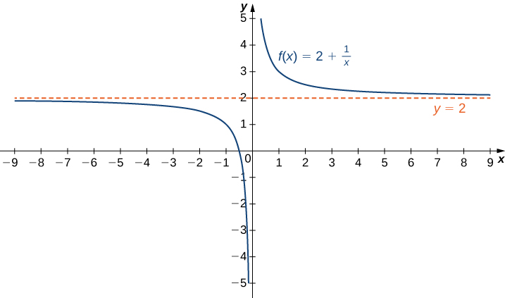
$x$	10	100	1,000	10,000
$2+\frac{1}{x}$	2.1	2.01	2.001	2.0001
$x$	−10	−100	−1000	−10,000
$2+\frac{1}{x}$	1.9	1.99	1.999	1.9999

More generally, for any function $f$, we say the limit as $x→∞$ of $f(x)$ is $L$ if $f(x)$ becomes arbitrarily close to $L$ as long as $x$ is sufficiently large. In that case, we write $\displaystyle \lim_{x→∞}f(x)=L$. Similarly, we say the limit as $x→−∞$ of $f(x)$ is $L$ if $f(x)$ becomes arbitrarily close to $L$ as long as $x<0$ and $|x|$ is sufficiently large. In that case, we write $\displaystyle \lim_{x→−∞}f(x)=L$. We now look at the definition of a function having a limit at infinity.

Definition: Limit at Infinity (Informal)

If the values of $f(x)$ become arbitrarily close to $L$ as $x$ becomes sufficiently large, we say the function $f$ has a limit at infinity and write

$$\lim_{x→∞}f(x)=L. \nonumber$$

If the values of $f(x)$ becomes arbitrarily close to $L$ for $x<0$ as $|x|$ becomes sufficiently large, we say that the function $f$ has a limit at negative infinity and write

$$\lim_{x→−∞}f(x)=L. \nonumber$$

If the values $f(x)$ are getting arbitrarily close to some finite value $L$ as $x→∞$ or $x→−∞$, the graph of $f$ approaches the line $y=L$. In that case, the line $y=L$ is a horizontal asymptote of $f$ (Figure $\PageIndex{2}$). For example, for the function $f(x)=\dfrac{1}{x}$, since $\displaystyle \lim_{x→∞}f(x)=0$, the line $y=0$ is a horizontal asymptote of $f(x)=\dfrac{1}{x}$.

Figure $\PageIndex{2}$: (a) As $x→∞$, the values of $f$ are getting arbitrarily close to $L$. The line $y=L$ is a horizontal asymptote of $f$. (b) As $x→−∞$, the values of $f$ are getting arbitrarily close to $M$. The line $y=M$ is a horizontal asymptote of $f$.

Definition: Horizontal Asymptote

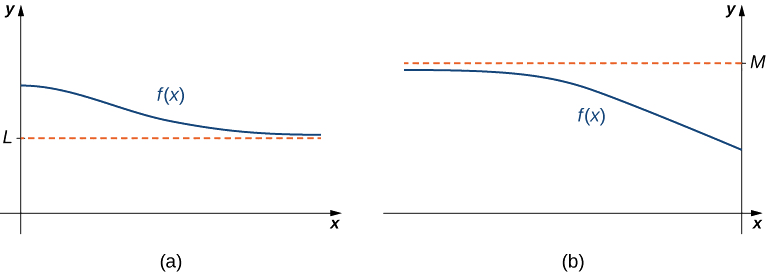
If $\displaystyle \lim_{x→∞}f(x)=L$ or $\displaystyle \lim_{x→−∞}f(x)=L$, we say the line $y=L$ is a horizontal asymptote of $f$.

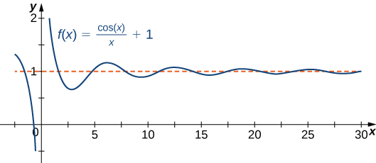
A function cannot cross a vertical asymptote because the graph must approach infinity (or $−∞$) from at least one direction as $x$ approaches the vertical asymptote. However, a function may cross a horizontal asymptote. In fact, a function may cross a horizontal asymptote an unlimited number of times. For example, the function $f(x)=\dfrac{\cos x}{x}+1$ shown in Figure $\PageIndex{3}$ intersects the horizontal asymptote $y=1$ an infinite number of times as it oscillates around the asymptote with ever-decreasing amplitude.

Figure $\PageIndex{3}$: The graph of $f(x)=(\cos x)/x+1$ crosses its horizontal asymptote $y=1$ an infinite number of times.

The algebraic limit laws and squeeze theorem we introduced in Introduction to Limits also apply to limits at infinity. We illustrate how to use these laws to compute several limits at infinity.

Example $\PageIndex{1}$: Computing Limits at Infinity

For each of the following functions $f$, evaluate $\displaystyle \lim_{x→∞}f(x)$ and $\displaystyle \lim_{x→−∞}f(x)$. Determine the horizontal asymptote(s) for $f$.

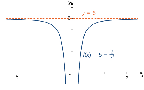
1. $f(x)=5−\dfrac{2}{x^2}$
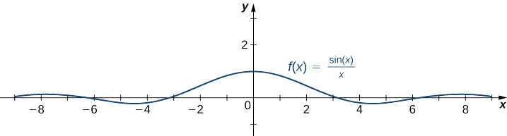
2. $f(x)=\dfrac{\sin x}{x}$
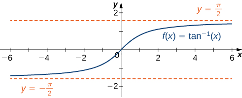
3. $f(x)=\tan^{−1}(x)$

Solution

a. Using the algebraic limit laws, we have

$$\lim_{x→∞}\left(5−\frac{2}{x^2}\right)=\lim_{x→∞}5−2\left(\lim_{x→∞}\frac{1}{x}\right)\cdot\left(\lim_{x→∞}\frac{1}{x}\right)=5−2⋅0=5.\nonumber$$

Similarly, $\displaystyle \lim_{x→−∞}f(x)=5$. Therefore, $f(x)=5-\dfrac{2}{x^2}$ has a horizontal asymptote of $y=5$ and $f$ approaches this horizontal asymptote as $x→±∞$ as shown in the following graph.

Figure $\PageIndex{4}$: This function approaches a horizontal asymptote as $x→±∞.$

b. Since $-1≤\sin x≤1$ for all $x$, we have

$$\frac{−1}{x}≤\frac{\sin x}{x}≤\frac{1}{x}\nonumber$$

for all $x≠0$. Also, since

$\displaystyle \lim_{x→∞}\frac{−1}{x}=0=\lim_{x→∞}\frac{1}{x}$,

we can apply the squeeze theorem to conclude that

$\displaystyle \lim_{x→∞}\frac{\sin x}{x}=0.$

Similarly,

$\displaystyle \lim_{x→−∞}\frac{\sin x}{x}=0.$

Thus, $f(x)=\dfrac{\sin x}{x}$ has a horizontal asymptote of $y=0$ and $f(x)$ approaches this horizontal asymptote as $x→±∞$ as shown in the following graph.

Figure $\PageIndex{5}$: This function crosses its horizontal asymptote multiple times.

c. To evaluate $\displaystyle \lim_{x→∞}\tan^{−1}(x)$ and $\displaystyle \lim_{x→−∞}\tan^{−1}(x)$, we first consider the graph of $y=\tan(x)$ over the interval $\left(−\frac{π}{2},\frac{π}{2}\right)$ as shown in the following graph.

Figure $\PageIndex{6}$: The graph of $y=\tan x$ has vertical asymptotes at $x=±\frac{π}{2}$

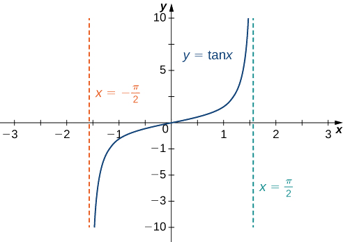
Since

$\displaystyle \lim_{x→\tfrac{π}{2}^−}\tan x=∞,$

it follows that

$\displaystyle \lim_{x→∞}\tan^{−1}(x)=\frac{π}{2}.$

Similarly, since

$\displaystyle \lim_{x→-\tfrac{π}{2}^+}\tan x=−∞,$

it follows that

$\displaystyle \lim_{x→−∞}\tan^{−1}(x)=−\frac{π}{2}.$

As a result, $y=\frac{π}{2}$ and $y=−\frac{π}{2}$ are horizontal asymptotes of $f(x)=\tan^{−1}(x)$ as shown in the following graph.

Figure $\PageIndex{7}$: This function has two horizontal asymptotes.

Exercise $\PageIndex{1}$

Evaluate $\displaystyle \lim_{x→−∞}\left(3+\frac{4}{x}\right)$ and $\displaystyle \lim_{x→∞}\left(3+\dfrac{4}{x}\right)$. Determine the horizontal asymptotes of $f(x)=3+\frac{4}{x},$ if any.

Hint

$\displaystyle \lim_{x→±∞}\frac{1}{x}=0$

Answer

Both limits are $3.$ The line $y=3$ is a horizontal asymptote.

Now we can consider an analytic process that may be needed to evaluate limits at infinity.  This process is often helpful when we have one of the indeterminate forms $\dfrac{±∞}{±∞}$.

Example $\PageIndex{2}$: A Process to Analytically Evaluate Limits at Infinity of Rational Functions

Determine the limit below, showing a clear analytic proof.

$\displaystyle \lim_{x \to \infty} \frac{x^2-2x+1}{4x^2 + 3}$

Solution

Note that evaluating the numerator and denominator of this expression at infinity gives us the form $\dfrac{∞}{∞}$.  This means a finite limit may exist, but it requires us to do some further work.  Since the expressions in the numerator and denominator are polynomials in this example, a process that will work here is to divide each term in the numerator and denominator by this variable raised to the highest power of the variable that we see in the denominator.

In this case, the highest power of the variable in the denominator is 2, so we divide through every term by $x^2$.

Note that we are really just multiplying the top and bottom of this expression by $\dfrac{1}{x^2}$, so this is not changing the value of the expression or the limit.

$\displaystyle \begin{align*} \lim_{x \to \infty} \frac{x^2-2x+1}{4x^2 + 3} &=  \lim_{x \to \infty} \frac{x^2-2x+1}{4x^2 + 3} \cdot \dfrac{\dfrac{1}{x^2}}{\dfrac{1}{x^2}} \\[5pt] &=  \lim_{x \to \infty} \dfrac{\dfrac{x^2}{x^2}-\dfrac{2x}{x^2}+\dfrac{1}{x^2}}{\dfrac{4x^2}{x^2} + \dfrac{3}{x^2}} \\[5pt] &=  \lim_{x \to \infty} \dfrac{1-\dfrac{2}{x}+\dfrac{1}{x^2}}{4 + \dfrac{3}{x^2}}  & & \text{Simplifying each term}\\[5pt] &=   \dfrac{\displaystyle \lim_{x \to \infty}\left(1-\dfrac{2}{x}+\dfrac{1}{x^2}\right)}{\displaystyle \lim_{x \to \infty}\left(4 + \dfrac{3}{x^2}\right)} & & \text{Using the Quotient Law for Limits.}\\[5pt] &= \dfrac{\displaystyle \lim_{x \to \infty} 1 -\lim_{x \to \infty} \dfrac{2}{x}+\lim_{x \to \infty} \dfrac{1}{x^2}}{\displaystyle \lim_{x \to \infty} 4 + \lim_{x \to \infty} \dfrac{3}{x^2}} & & \text{Using the Sum/Difference Laws for Limits.}\\[5pt] &= \dfrac{\displaystyle 1 - \cancelto{0} {\lim_{x \to \infty} \dfrac{2}{x}} + \cancelto{0} {\lim_{x \to \infty} \dfrac{1}{x^2}}}{\displaystyle  4 +  \cancelto{0} {\lim_{x \to \infty} \dfrac{3}{x^2}}} & & \text{Using limits we know.}\\[5pt] &= \dfrac{1}{4}\end{align*}$

Thus we have proven this limit is $\dfrac{1}{4}$.

We also know that $f(x) = \dfrac{x^2-2x+1}{4x^2 + 3}$ has a horizontal asymptote of $y = \dfrac{1}{4}$ as $x→∞$.

Note that in Example $\PageIndex{2}$, since the degree of the polynomials in the numerator and denominator were the same, the limit as $x→∞$ ends up being the ratio of the coefficients of the terms of highest (matching) degree in the numerator and denominator.  This will be true generally, but a proof like that shown here may still required to be shown.  However, it is not always necessary to show all the steps shown in Example $\PageIndex{2}$.  In the next example, we will show how an abbreviated process can be used to determine the limits of rational functions of this type, as $x$ approaches infinity.

Example $\PageIndex{3}$ 

Determine the limits below, showing a clear analytic proof of each.

a. $\displaystyle \lim_{x \to \infty} \frac{2x^2-4x}{5x^3 - 7}$

b. $\displaystyle \lim_{x \to \infty} \frac{\sqrt{2x^2-1}}{5x +2}$

Solution

a. We see that this limit again has the form $\dfrac{∞}{∞}$.  If it did not, we would evaluate the limit using a different approach.

We start be dividing all terms in the numerator and denominator by $x^3$, the highest power of $x$ found in the denominator.  Then we will proceed as we did in Example $\PageIndex{2}$, except that we will only include the most important steps this time.

$\displaystyle \begin{align*} \lim_{x \to \infty} \frac{2x^2-4x}{5x^3 - 7} &=  \lim_{x \to \infty} \dfrac{\dfrac{2x^2}{x^3}-\dfrac{4x}{x^3}}{\dfrac{5x^3}{x^3} - \dfrac{7}{x^3}} & & \text{Dividing each term by the highest power of }x\text{ in the denominator.} \\[5pt] &=  \lim_{x \to \infty} \dfrac{\dfrac{2}{x}-\dfrac{4}{x^2}}{5 - \dfrac{7}{x^3}}  & & \text{Simplifying each term}\\[5pt] &= \lim_{x \to \infty} \dfrac{\cancelto{0} {\dfrac{2}{x}}-\cancelto{0} {\dfrac{4}{x^2}}}{5 - \cancelto{0} {\dfrac{7}{x^3}}} & & \text{Considering where each term will go as }x→∞ \\[5pt] &= \dfrac{0}{5} \\[5pt] &= 0 \end{align*}$

We have proven this limit is $0$ and that $f(x) = \dfrac{2x^2-4x}{5x^3 - 7}$ has a horizontal asymptote of $y = 0$ as $x→∞$.

b. Now let's consider $\displaystyle \lim_{x \to \infty} \frac{\sqrt{2x^2-1}}{5x +2}$.

The rational function in this limit is different since it has a square root in it, but it turns out that we can use the same approach to evaluate this limit that we have been using in Example $\PageIndex{2}$ and Example $\PageIndex{3a}$.

First, consider the "net degree" of the numerator of this expression.  The highest degree term under the radical is $2x^2$.  Since it's under a radical, it's "net degree" can be found by simplifying this term.  That is, $\sqrt{2x^2} = \sqrt{2} \sqrt{x^2} = \sqrt{2} (x^2)^{1/2} = \left(\sqrt{2}\right)\; x$, if $x>0$.  That is, the numerator has a net degree of $1$!

Since the degrees of the numerator and denominator are both $1$, we anticipate a finite limit related to the coefficients of the two terms of highest degree.  Let's see how the work plays out in this example.

$\displaystyle \begin{align*} \lim_{x \to \infty} \frac{\sqrt{2x^2-1}}{5x +2} &=  \lim_{x \to \infty} \dfrac{\dfrac{\sqrt{2x^2-1}}{x}}{\dfrac{5x}{x} +\dfrac{2}{x}} & & \text{Dividing each term by the highest power of }x\text{ in the denominator.} \\[5pt] &=  \lim_{x \to \infty} \dfrac{\sqrt{\dfrac{2x^2}{x^2}-\dfrac{1}{x^2}}}{\dfrac{5x}{x} +\dfrac{2}{x}}   & & \text{Bringing the }x\text{ inside the radical.}\\[5pt] &=  \lim_{x \to \infty} \dfrac{\sqrt{2-\dfrac{1}{x^2}}}{5 +\dfrac{2}{x}}   & & \text{Simplifying each term.}\\[5pt] &= \lim_{x \to \infty} \dfrac{\sqrt{2 - \cancelto{0} {\dfrac{1}{x^2}}}}{5 + \cancelto{0} {\dfrac{2}{x}}} & & \text{Considering where each term will go as }x→∞ \\[5pt] &= \dfrac{\sqrt{2}}{5} \end{align*}$

Thus, this limit is $\dfrac{\sqrt{2}}{5}$, and the function $f(x) = \dfrac{\sqrt{2x^2-1}}{5x +2}$ has a horizontal asymptote of $y = \dfrac{\sqrt{2}}{5}$ as $x→∞$.

We see in Example $\PageIndex{3a}$ that when the degree of the denominator is larger than the degree of the numerator, the limit will be $0$ as $x→∞$.

In Example $\PageIndex{4}$ below, we will consider what happens when the degree of the numerator is larger than the degree of the denominator.  But first, we must consider another possible value for a limit.

Infinite Limits at Infinity

Sometimes the values of a function $f$ become arbitrarily large as $x→∞$(or as $x→−∞$). In this case, we write $\displaystyle \lim_{x→∞}f(x)=∞$ (or $\displaystyle \lim_{x→−∞}f(x)=∞$). On the other hand, if the values of $f$ are negative but become arbitrarily large in magnitude as $x→∞$ (or as $x→−∞$), we write $\displaystyle \lim_{x→∞}f(x)=−∞$ (or $\displaystyle \lim_{x→−∞}f(x)=−∞$).

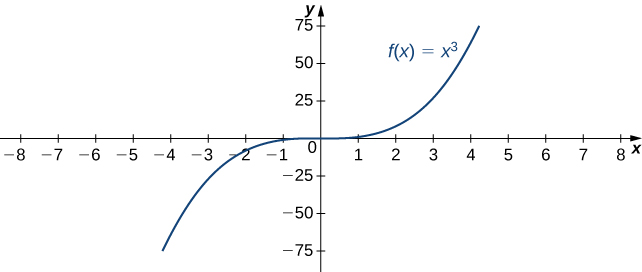
For example, consider the function $f(x)=x^3$. As seen in Table $\PageIndex{2}$ and Figure $\PageIndex{8}$, as $x→∞$ the values $f(x)$ become arbitrarily large. Therefore, $\displaystyle \lim_{x→∞}x^3=∞$. On the other hand, as $x→−∞$, the values of $f(x)=x^3$ are negative but become arbitrarily large in magnitude. Consequently, $\displaystyle \lim_{x→−∞}x^3=−∞.$

Table $\PageIndex{2}$: Values of a power function as $x→±∞$

$x$	10	20	50	100	1000
$x^3$	1000	8000	125,000	1,000,000	1,000,000,000
$x$	−10	−20	−50	−100	−1000
$x^3$	−1000	−8000	−125,000	−1,000,000	−1,000,000,000

Figure $\PageIndex{8}$: For this function, the functional values approach $±$infinity as $x→±∞.$

Definition: Infinite Limit at Infinity (Informal)

We say a function $f$ has an infinite limit at infinity and write

$$\lim_{x→∞}f(x)=∞. \nonumber$$

if $f(x)$ becomes arbitrarily large for $x$ sufficiently large. We say a function has a negative infinite limit at infinity and write

$$\lim_{x→∞}f(x)=−∞. \nonumber$$

if $f(x)<0$ and $|f(x)|$ becomes arbitrarily large for $x$ sufficiently large. Similarly, we can define infinite limits as $x→−∞.$

Example $\PageIndex{4}$

Determine the following limit, showing a clear analytic proof.

$\displaystyle \lim_{x \to \infty} \frac{x^5-3x+4}{10x^3 + x^2 - 1}$

Solution

Since this limit has the form $\dfrac{∞}{∞}$, we proceed as we did in Examples $\PageIndex{2}$ and $\PageIndex{3}$, first dividing each term by $x^3$, the highest power of $x$ in the denominator of this rational expression.

$\displaystyle \begin{align*} \lim_{x \to \infty} \frac{x^5-3x+4}{10x^3 + x^2 - 1} &=  \lim_{x \to \infty} \dfrac{\dfrac{x^5}{x^3}-\dfrac{3x}{x^3} + \dfrac{4}{x^3}}{\dfrac{10x^3}{x^3} + \dfrac{x^2}{x^3} - \dfrac{1}{x^3}} & & \text{Dividing each term by the highest power of }x\text{ in the denominator.} \\[5pt] &=  \lim_{x \to \infty} \dfrac{x^2-\dfrac{3}{x^2} + \dfrac{4}{x^3}}{10 + \dfrac{1}{x} - \dfrac{1}{x^3}}  & & \text{Simplifying each term}\\[5pt] &= \lim_{x \to \infty} \dfrac{x^2-\cancelto{0} {\dfrac{3}{x^2}} + \cancelto{0} {\dfrac{4}{x^3}}}{10 + \cancelto{0} {\dfrac{1}{x}} - \cancelto{0} {\dfrac{1}{x^3}}} & & \text{Considering where each term will go as }x→∞ \\[5pt] &= \lim_{x \to \infty} \dfrac{x^2}{10} \\[5pt] &= \infty \end{align*}$

So, in this case, the limit is not finite.  We say that, $\displaystyle \lim_{x \to \infty} \frac{x^5-3x+4}{10x^3 + x^2 - 1} = \infty$.

Therefore the function $f(x) = \dfrac{x^5-3x+4}{10x^3 + x^2 - 1}$ has no horizontal asymptote as $x→∞$.

 So we see that when the degree of the numerator is larger than the degree of the denominator, the limit as $x→∞$ is either $\infty$ or $-\infty$.  (How would it become $-\infty$?)

Formal Definitions

Earlier, we used the terms arbitrarily close, arbitrarily large, and sufficiently large to define limits at infinity informally. Although these terms provide accurate descriptions of limits at infinity, they are not precise mathematically. Here are more formal definitions of limits at infinity. We then look at how to use these definitions to prove results involving limits at infinity.

Definition: Limit at Infinity (Formal)

We say a function $f$ has a limit at infinity, if there exists a real number $L$ such that for all $ε>0$, there exists $N>0$ such that

$$|f(x)−L|<ε \nonumber$$

for all $x>N.$ in that case, we write

$$\lim_{x→∞}f(x)=L \nonumber$$

Figure $\PageIndex{9}$: For a function with a limit at infinity, for all $x>N, |f(x)−L|<ε.$

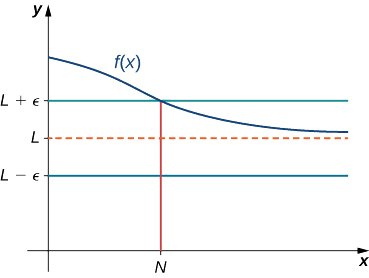
Earlier in this section, we used graphical evidence in Figure $\PageIndex{1}$ and numerical evidence in Table $\PageIndex{1}$ to conclude that $\displaystyle \lim_{x→∞}\left(2+\frac{1}{x}\right)=2$. Here we use the formal definition of limit at infinity to prove this result rigorously.

Example $\PageIndex{5}$:

Use the formal definition of limit at infinity to prove that $\displaystyle \lim_{x→∞}\left(2+\frac{1}{x}\right)=2$.

Solution

Let $ε>0.$ Let $N=\frac{1}{ε}$. Therefore, for all $x>N$, we have

$$\left|2+\frac{1}{x}−2\right|=\left|\frac{1}{x}\right|=\frac{1}{x}<\frac{1}{N}=ε \nonumber$$

Exercise $\PageIndex{2}$

Use the formal definition of limit at infinity to prove that $\displaystyle \lim_{x→∞}\left(3-\frac{1}{x^2}\right)=3$.

Hint

Let $N=\frac{1}{\sqrt{ε}}$.

Answer

Let $ε>0.$ Let $N=\frac{1}{\sqrt{ε}}$. Therefore, for all $x>N,$ we have

$$\Big|3−\frac{1}{x^2}−3\Big|=\frac{1}{x^2}<\frac{1}{N^2}=ε \nonumber$$

Therefore, $\displaystyle \lim_{x→∞}(3−1/x^2)=3.$

We now turn our attention to a more precise definition for an infinite limit at infinity.

Definition: Infinite Limit at Infinity (Formal)

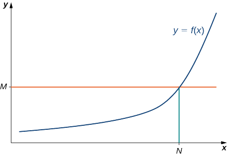
We say a function $f$ has an infinite limit at infinity and write

$\displaystyle \lim_{x→∞}f(x)=∞$

if for all $M>0,$ there exists an $N>0$ such that

$f(x)>M$

for all $x>N$ (see Figure $\PageIndex{10}$).

We say a function has a negative infinite limit at infinity and write

$\displaystyle \lim_{x→∞}f(x)=−∞$

if for all $M<0$, there exists an $N>0$ such that

$f(x)<M$

for all $x>N$.

Similarly we can define limits as $x→−∞.$

Figure $\PageIndex{10}$: For a function with an infinite limit at infinity, for all $x>N,\; f(x)>M.$

Earlier, we used graphical evidence (Figure $\PageIndex{8}$) and numerical evidence (Table $\PageIndex{2}$) to conclude that $\displaystyle \lim_{x→∞}x^3=∞$. Here we use the formal definition of infinite limit at infinity to prove that result.

Example $\PageIndex{6}$

Use the formal definition of infinite limit at infinity to prove that $\displaystyle \lim_{x→∞}x^3=∞.$

Solution

Let $M>0.$ Let $N=\sqrt[3]{M}$. Then, for all $x>N$, we have

$x^3>N^3=(\sqrt[3]{M})^3=M.$

Therefore, $\displaystyle \lim_{x→∞}x^3=∞$.

Exercise $\PageIndex{3}$

Use the formal definition of infinite limit at infinity to prove that $\displaystyle \lim_{x→∞}3x^2=∞.$

Hint

Let $N=\sqrt{\frac{M}{3}}$.

Answer

Let $M>0.$ Let $N=\sqrt{\frac{M}{3}}$. Then, for all $x>N,$ we have

$3x^2>3N^2=3\left(\sqrt{\frac{M}{3}}\right)^2=\frac{3M}{3}=M$

Key Concepts

• The limit of $f(x)$ is $L$ as $x→∞$ (or as $x→−∞)$ if the values $f(x)$ become arbitrarily close to $L$ as $x$ becomes sufficiently large.
• The limit of $f(x)$ is $∞$ as $x→∞$ if $f(x)$ becomes arbitrarily large as $x$ becomes sufficiently large. The limit of $f(x)$ is $−∞$ as $x→∞$ if $f(x)<0$ and $|f(x)|$ becomes arbitrarily large as $x$ becomes sufficiently large. We can define the limit of $f(x)$ as $x$ approaches $−∞$ similarly.

Glossary

horizontal asymptote

if $\displaystyle \lim_{x→∞}f(x)=L$ or $\displaystyle \lim_{x→−∞}f(x)=L$, then $y=L$ is a horizontal asymptote of $f$

infinite limit at infinity

a function that becomes arbitrarily large as $x$ becomes large

limit at infinity

a function that approaches a limit value $L$ as $x$ becomes large

Contributors and Attributions

• Gilbert Strang (MIT) and Edwin “Jed” Herman (Harvey Mudd) with many contributing authors. This content by OpenStax is licensed with a CC-BY-SA-NC 4.0 license. Download for free at http://cnx.org.

• Paul Seeburger (Monroe Community College) added Examples $\PageIndex{2}$, $\PageIndex{3}$, and $\PageIndex{4}$ and the discussion just preceding and after each.