The notation refers to the collection of ordered lists of real numbers, that is In this chapter, we take a closer look at vectors in . First, we will consider what looks like in more detail. Recall that the point given by is called the origin.
Now, consider the case of for Then from the definition we can identify with points in as follows: Hence, is defined as the set of all real numbers and geometrically, we can describe this as all the points on a line.
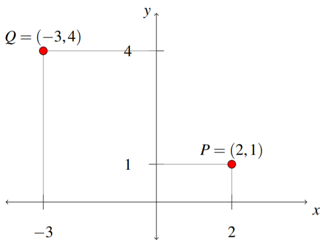
Now suppose . Then, from the definition, Consider the familiar coordinate plane, with an axis and a axis. Any point within this coordinate plane is identified by where it is located along the axis, and also where it is located along the axis. Consider as an example the following diagram.
Figure
Hence, every element in is identified by two components, and , in the usual manner. The coordinates (or ,) uniquely determine a point in the plan. Note that while the definition uses and to label the coordinates and you may be used to and , these notations are equivalent.
Now suppose . You may have previously encountered the -dimensional coordinate system, given by
Points in will be determined by three coordinates, often written which correspond to the , , and axes. We can think as above that the first two coordinates determine a point in a plane. The third component determines the height above or below the plane, depending on whether this number is positive or negative, and all together this determines a point in space. You see that the ordered triples correspond to points in space just as the ordered pairs correspond to points in a plane and single real numbers correspond to points on a line.
The idea behind the more general is that we can extend these ideas beyond This discussion regarding points in leads into a study of vectors in . While we consider for all , we will largely focus on in this section.
Consider the following definition.
Definition The Position Vector
Let be the coordinates of a point in Then the vector with its tail at and its tip at is called the position vector of the point . We write
For this reason we may write both and .
This definition is illustrated in the following picture for the special case of .
Figure
Thus every point in determines its position vector . Conversely, every such position vector which has its tail at and point at determines the point of .
Now suppose we are given two points, whose coordinates are and respectively. We can also determine the position vector from to (also called the vector from to ) defined as follows.
Now, imagine taking a vector in and moving it around, always keeping it pointing in the same direction as shown in the following picture.
Figure
After moving it around, it is regarded as the same vector. Each vector, and has the same length (or magnitude) and direction. Therefore, they are equal.
Consider now the general definition for a vector in .
Definition Vectors in
Let Then, is called a vector. Vectors have both size (magnitude) and direction. The numbers are called the components of .
Using this notation, we may use to denote the position vector of point . Notice that in this context, . These notations may be used interchangeably.
You can think of the components of a vector as directions for obtaining the vector. Consider . Draw a vector with its tail at the point and its tip at the point . This vector it is obtained by starting at , moving parallel to the axis to and then from here, moving parallel to the axis to and finally parallel to the axis to Observe that the same vector would result if you began at the point , moved parallel to the axis to then parallel to the axis to and finally parallel to the axis to . Here, the vector would have its tail sitting at the point determined by and its point at It is the same vector because it will point in the same direction and have the same length. It is like you took an actual arrow, and moved it from one location to another keeping it pointing the same direction.
We conclude this section with a brief discussion regarding notation. In previous sections, we have written vectors as columns, or matrices. For convenience in this chapter we may write vectors as the transpose of row vectors, or matrices. These are of course equivalent and we may move between both notations. Therefore, recognize that
Notice that two vectors and are equal if and only if all corresponding components are equal. Precisely, Thus and but because, even though the same numbers are involved, the order of the numbers is different.
For the specific case of , there are three special vectors which we often use. They are given by We can write any vector as a linear combination of these vectors, written as . This notation will be used throughout this chapter.
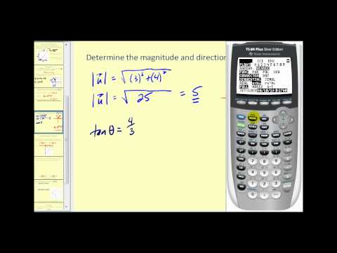
Below is a video on vectors in 2D.
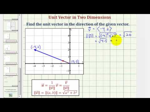
Below is a video on finding a unit vector given the graph of a vector in 2D.
Below is a video on finding the component form of a vector from its graph.


![Plot of P=(p1,p2,p3) and line segment 0P =[p1 p2 p3]^T and the axes shown.](https://math.libretexts.org/@api/deki/files/74969/clipboard_e82b8a22c24a336d00c9648a43c016dda.png?revision=1)
![Plot of vector 0P = [p1,p2,p3] from (0,0,0) to (p1,p2,p3). Also plotted is vector AB which is vector OP shifted up and left.](https://math.libretexts.org/@api/deki/files/74970/clipboard_e29d116f1c6f05217e46dd0513baacdbf.png?revision=1)