5.4: Special Linear Transformations in R²

Outcomes

1. Find the matrix of rotations and reflections in $\mathbb{R}^2$ and determine the action of each on a vector in $\mathbb{R}^2$.

In this section, we will examine some special examples of linear transformations in $\mathbb{R}^2$ including rotations and reflections. We will use the geometric descriptions of vector addition and scalar multiplication discussed earlier to show that a rotation of vectors through an angle and reflection of a vector across a line are examples of linear transformations.

More generally, denote a transformation given by a rotation by $T$. Why is such a transformation linear? Consider the following picture which illustrates a rotation. Let $\vec{u},\vec{v}$ denote vectors.

Figure $\PageIndex{1}$

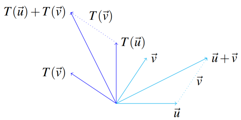
Let’s consider how to obtain $T\left [ \vec{u}+\vec{v}\right ]$. Simply, you add $T (\vec{u})$ and $T(\vec{v})$. Here is why. If you add $T(\vec{u})$ to $T(\vec{v})$ you get the diagonal of the parallelogram determined by $T(\vec{u})$ and $T(\vec{v})$, as this action is our usual vector addition. Now, suppose we first add $\vec{u}$ and $\vec{v}$, and then apply the transformation $T$ to $\vec{u}+\vec{v}$. Hence, we find $T( \vec{u}+\vec{v})$. As shown in the diagram, this will result in the same vector. In other words, $T(\vec{u}+\vec{v}) = T(\vec{u}) + T(\vec{v})$.

This is because the rotation preserves all angles between the vectors as well as their lengths. In particular, it preserves the shape of this parallelogram. Thus both $T\left [\vec{u}\right ]+T\left [\vec{v}\right ]$ and $T\left [\vec{u}+\vec{v}\right ]$ give the same vector. It follows that $T$ distributes across addition of the vectors of $\mathbb{R}^{2}$.

Similarly, if $k$ is a scalar, it follows that $T\left [k\vec{u}\right ]=kT\left [\vec{u}\right ]$. Thus rotations are an example of a linear transformation by Definition 9.6.1.

The following theorem gives the matrix of a linear transformation which rotates all vectors through an angle of $\theta$.

Theorem $\PageIndex{1}$:Rotation

Let $R_{\theta}: \mathbb{R}^2 \to \mathbb{R}^2$ be a linear transformation given by rotating vectors through an angle of $\theta$. Then the matrix $A$ of $R_{\theta}$ is given by $$\left [ \begin{array}{rr} \cos \left [ \theta \right ] & -\sin \left [ \theta \right ] \\ \sin \left [ \theta \right ] & \cos \left [ \theta \right ] \end{array} \right ]\nonumber$$

Proof

Let $\vec{e}_{1} = \left [ \begin{array}{r} 1 \\ 0 \end{array} \right ]$ and $\vec{e}_{2} = \left [ \begin{array}{r} 0 \\ 1 \end{array} \right ] .$ These identify the geometric vectors which point along the positive $x$ axis and positive $y$ axis as shown.

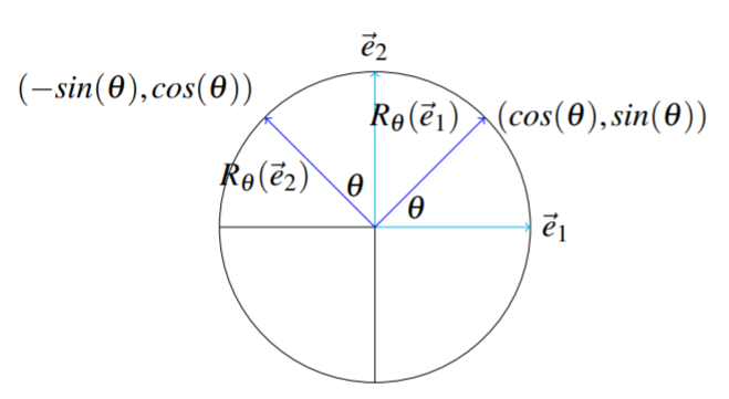
Figure $\PageIndex{2}$

From Theorem 5.2.2, we need to find $R_{\theta}(\vec{e}_{1})$ and $R_{\theta}(\vec{e}_{2}),$ and use these as the columns of the matrix $A$ of $T$. We can use $\cos, \sin$ of the angle $\theta$ to find the coordinates of $R_{\theta}(\vec{e}_{1})$ as shown in the above picture. The coordinates of $R_{\theta}(\vec{e}_{2})$ also follow from trigonometry. Thus $$R_{\theta}(\vec{e}_{1})=\left [ \begin{array}{r} \cos \theta \\ \sin \theta \end{array} \right ] ,R_{\theta}(\vec{e}_{2})=\left [ \begin{array}{r} -\sin \theta \\ \cos \theta \end{array} \right ]\nonumber$$ Therefore, from Theorem 5.2.2, $$A=\left [ \begin{array}{rr} \cos \theta & -\sin \theta \\ \sin \theta & \cos \theta \end{array} \right ]\nonumber$$

We can also prove this algebraically without the use of the above picture. The definition of $\left [ \cos \left [ \theta \right ] ,\sin \left [ \theta \right ] \right ]$ is as the coordinates of the point of $R_{\theta}(\vec{e}_{1})$. Now the point of the vector $\vec{e}_{2}$ is exactly $\pi /2$ further along the unit circle from the point of $\vec{e}_{1}$, and therefore after rotation through an angle of $\theta$ the coordinates $x$ and $y$ of the point of $R_{\theta}(\vec{e}_{2})$ are given by $$\left [ x,y\right ] =\left [ \cos \left [ \theta +\pi /2\right ] ,\sin \left [ \theta +\pi /2\right ] \right ] =\left [ -\sin \theta ,\cos \theta \right ]\nonumber$$

Consider the following example.

Example $\PageIndex{1}$:Rotation in $\mathbb{R}^2$

Let $R_{\frac{\pi}{2}}: \mathbb{R}^2 \to \mathbb{R}^2$ denote rotation through $\pi/2$. Find the matrix of $R_{\frac{\pi}{2}}$. Then, find $R_{\frac{\pi}{2}} (\vec{x})$ where $\vec{x} = \left [ \begin{array}{r} 1 \\ -2 \end{array} \right ]$.

Solution

By Theorem $\PageIndex{1}$, the matrix of $R_{\frac{\pi}{2}}$ is given by $$\left [ \begin{array}{rr} \cos \left [ \theta \right ] & -\sin \left [ \theta \right ] \\ \sin \left [ \theta \right ] & \cos \left [ \theta \right ] \end{array} \right ] = \left [ \begin{array}{rr} \cos \left [ \pi/2 \right ] & -\sin \left [ \pi/2 \right ] \\ \sin \left [ \pi/2 \right ] & \cos \left [ \pi/2 \right ] \end{array} \right ] = \left [ \begin{array}{rr} 0 & -1 \\ 1 & 0 \end{array} \right ]\nonumber$$

To find $R_{\frac{\pi}{2}} (\vec{x})$, we multiply the matrix of $R_{\frac{\pi}{2}}$ by $\vec{x}$ as follows $$\left [ \begin{array}{rr} 0 & -1 \\ 1 & 0 \end{array} \right ] \left [ \begin{array}{r} 1 \\ -2 \end{array} \right ] = \left [ \begin{array}{r} 2 \\ 1 \end{array} \right ]\nonumber$$

Below is a video on finding the transformation matrix ifor a 2D rotation.

We now look at an example of a linear transformation involving two angles.

Example $\PageIndex{2}$:The Rotation Matrix of the Sum of Two Angles

Find the matrix of the linear transformation which is obtained by first rotating all vectors through an angle of $\phi$ and then through an angle $\theta .$ Hence the linear transformation rotates all vectors through an angle of $\theta +\phi .$

Solution

Let $R_{\theta +\phi }$ denote the linear transformation which rotates every vector through an angle of $\theta +\phi .$ Then to obtain $R_{\theta +\phi },$ we first apply $R_{\phi }$ and then $R_{\theta }$ where $R_{\phi }$ is the linear transformation which rotates through an angle of $\phi$ and $R_{\theta }$ is the linear transformation which rotates through an angle of $\theta$. Denoting the corresponding matrices by $A_{\theta +\phi }$, $A_{\phi },$ and $A_{\theta },$ it follows that for every $\vec{u}$ $$R_{\theta +\phi }\left [\vec{u}\right ]=A_{\theta +\phi }\vec{u}=A_{\theta }A_{\phi }\vec{u} = R_{\theta }R_{\phi } \left [\vec{u}\right ]\nonumber$$ Notice the order of the matrices here!

Consequently, you must have $$\begin{aligned} A_{\theta +\phi } &=\left [ \begin{array}{cc} \cos \left [ \theta +\phi \right ] & -\sin \left [ \theta +\phi \right ] \\ \sin \left [ \theta +\phi \right ] & \cos \left [ \theta +\phi \right ] \end{array} \right ]\\ &=\left [ \begin{array}{cc} \cos \theta & -\sin \theta \\ \sin \theta & \cos \theta \end{array} \right ] \left [ \begin{array}{cc} \cos \phi & -\sin \phi \\ \sin \phi & \cos \phi \end{array} \right ] =A_{\theta }A_{\phi } \end{aligned}$$

The usual matrix multiplication yields $$\begin{aligned} A_{\theta +\phi } &= \left [ \begin{array}{cc} \cos \left [ \theta +\phi \right ] & -\sin \left [ \theta +\phi \right ] \\ \sin \left [ \theta +\phi \right ] & \cos \left [ \theta +\phi \right ] \end{array} \right ] \\ &=\left [ \begin{array}{cc} \cos \theta \cos \phi -\sin \theta \sin \phi & -\cos \theta \sin \phi -\sin \theta \cos \phi \\ \sin \theta \cos \phi +\cos \theta \sin \phi & \cos \theta \cos \phi -\sin \theta \sin \phi \end{array} \right ] \\ &= A_{\theta }A_{\phi } \end{aligned}$$

Don’t these look familiar? They are the usual trigonometric identities for the sum of two angles derived here using linear algebra concepts.

Here we have focused on rotations in two dimensions. However, you can consider rotations and other geometric concepts in any number of dimensions. This is one of the major advantages of linear algebra. You can break down a difficult geometrical procedure into small steps, each corresponding to multiplication by an appropriate matrix. Then by multiplying the matrices, you can obtain a single matrix which can give you numerical information on the results of applying the given sequence of simple procedures.

Linear transformations which reflect vectors across a line are a second important type of transformations in $\mathbb{R}^2$. Consider the following theorem.

Theorem $\PageIndex{2}$:Reflection

Let $Q_m: \mathbb{R}^2 \to \mathbb{R}^2$ be a linear transformation given by reflecting vectors over the line $\vec{y}=m\vec{x}$. Then the matrix of $Q_m$ is given by $$\frac{1}{1+m^2} \left [ \begin{array}{cc} 1-m^2 & 2m \\ 2m & m^2-1 \end{array} \right ]\nonumber$$

Consider the following example.

Example $\PageIndex{3}$:Reflection in $\mathbb{R}^2$

Let $Q_2: \mathbb{R}^2 \to \mathbb{R}^2$ denote reflection over the line $\vec{y}=2\vec{x}$. Then $Q_2$ is a linear transformation. Find the matrix of $Q_2$. Then, find $Q_2 (\vec{x})$ where $\vec{x} = \left [ \begin{array}{r} 1 \\ -2 \end{array} \right ]$.

Solution

By Theorem $\PageIndex{2}$, the matrix of $Q_2$ is given by $$\frac{1}{1+m^2} \left [ \begin{array}{cc} 1-m^2 & 2m \\ 2m & m^2-1 \end{array} \right ] = \frac{1}{1+(2)^2} \left [ \begin{array}{cc} 1-(2)^2 & 2(2) \\ 2(2) & (2)^2-1 \end{array} \right ] = \frac{1}{5} \left [ \begin{array}{rr} -3 & 8 \\ 8 & 3 \end{array} \right ]\nonumber$$

To find $Q_2(\vec{x})$ we multiply $\vec{x}$ by the matrix of $Q_2$ as follows: $$\frac{1}{5} \left [ \begin{array}{rr} -3 & 8 \\ 8 & 3 \end{array} \right ] \left [ \begin{array}{r} 1 \\ -2 \end{array} \right ] = \left [ \begin{array}{r} - \frac{19}{5} \\ \frac{2}{5} \end{array} \right ]\nonumber$$

Below is a video on sketching a linear transformation of a rectangle given the transformation matrix (reflection).

Consider the following example which incorporates a reflection as well as a rotation of vectors.

Example $\PageIndex{4}$:Rotation Followed by a Reflection

Find the matrix of the linear transformation which is obtained by first rotating all vectors through an angle of $\pi /6$ and then reflecting through the $x$ axis.

Solution

By Theorem $\PageIndex{1}$, the matrix of the transformation which involves rotating through an angle of $\pi /6$ is $$\left [ \begin{array}{rr} \cos \left [ \pi /6\right ] & -\sin \left [ \pi /6\right ] \\ \sin \left [ \pi /6\right ] & \cos \left [ \pi /6\right ] \end{array} \right ] =\left [ \begin{array}{cc} \frac{1}{2}\sqrt{3} & - \frac{1}{2} \\ \frac{1}{2} & \frac{1}{2}\sqrt{3} \end{array} \right ]\nonumber$$

Reflecting across the $x$ axis is the same action as reflecting vectors over the line $\vec{y}=m\vec{x}$ with $m=0$. By Theorem $\PageIndex{2}$, the matrix for the transformation which reflects all vectors through the $x$ axis is $$\frac{1}{1+m^2} \left [ \begin{array}{cc} 1-m^2 & 2m \\ 2m & m^2-1 \end{array} \right ] = \frac{1}{1+(0)^2} \left [ \begin{array}{cc} 1-(0)^2 & 2(0) \\ 2(0) & (0)^2-1 \end{array} \right ] = \left [ \begin{array}{rr} 1 & 0 \\ 0 & -1 \end{array} \right ]\nonumber$$

Therefore, the matrix of the linear transformation which first rotates through $\pi /6$ and then reflects through the $x$ axis is given by $$\left [ \begin{array}{rr} 1 & 0 \\ 0 & -1 \end{array} \right ] \left [ \begin{array}{rr} \frac{1}{2}\sqrt{3} & - \frac{1}{2} \\ \frac{1}{2} & \frac{1}{2}\sqrt{3} \end{array} \right ] = \ \left [ \begin{array}{rr} \frac{1}{2}\sqrt{3} & - \frac{1}{2} \\ - \frac{1}{2} & - \frac{1}{2}\sqrt{3} \end{array} \right ]\nonumber$$

Below is a video on describing the range or image of a linear transformation (line reflection).