7.1: Eigenvalues and Eigenvectors of a Matrix

Outcomes

1. Describe eigenvalues geometrically and algebraically.
2. Find eigenvalues and eigenvectors for a square matrix.

Spectral Theory refers to the study of eigenvalues and eigenvectors of a matrix. It is of fundamental importance in many areas and is the subject of our study for this chapter.

Definition of Eigenvectors and Eigenvalues

In this section, we will work with the entire set of complex numbers, denoted by $\mathbb{C}$. Recall that the real numbers, $\mathbb{R}$ are contained in the complex numbers, so the discussions in this section apply to both real and complex numbers.

To illustrate the idea behind what will be discussed, consider the following example.

Example $\PageIndex{1}$:Eigenvectors and Eigenvalues

Let $$A = \left[ \begin{array}{rrr} 0 & 5 & -10 \\ 0 & 22 & 16 \\ 0 & -9 & -2 \end{array} \right]\nonumber$$ Compute the product $AX$ for $$X = \left[ \begin{array}{r} -5 \\ -4 \\ 3 \end{array} \right], X = \left[ \begin{array}{r} 1 \\ 0 \\ 0 \end{array} \right]\nonumber$$ What do you notice about $AX$ in each of these products?

Solution

First, compute $AX$ for $$X =\left[ \begin{array}{r} -5 \\ -4 \\ 3 \end{array} \right]\nonumber$$

This product is given by $$AX = \left[ \begin{array}{rrr} 0 & 5 & -10 \\ 0 & 22 & 16 \\ 0 & -9 & -2 \end{array} \right] \left[ \begin{array}{r} -5 \\ -4 \\ 3 \end{array} \right] = \left[ \begin{array}{r} -50 \\ -40 \\ 30 \end{array} \right] =10\left[ \begin{array}{r} -5 \\ -4 \\ 3 \end{array} \right]\nonumber$$

In this case, the product $AX$ resulted in a vector which is equal to $10$ times the vector $X$. In other words, $AX=10X$.

Let’s see what happens in the next product. Compute $AX$ for the vector $$X = \left[ \begin{array}{r} 1 \\ 0 \\ 0 \end{array} \right]\nonumber$$

This product is given by $$AX = \left[ \begin{array}{rrr} 0 & 5 & -10 \\ 0 & 22 & 16 \\ 0 & -9 & -2 \end{array} \right] \left[ \begin{array}{r} 1 \\ 0 \\ 0 \end{array} \right] = \left[ \begin{array}{r} 0 \\ 0 \\ 0 \end{array} \right] =0\left[ \begin{array}{r} 1 \\ 0 \\ 0 \end{array} \right]\nonumber$$

In this case, the product $AX$ resulted in a vector equal to $0$ times the vector $X$, $AX=0X$.

Perhaps this matrix is such that $AX$ results in $kX$, for every vector $X$. However, consider $$\left[ \begin{array}{rrr} 0 & 5 & -10 \\ 0 & 22 & 16 \\ 0 & -9 & -2 \end{array} \right] \left[ \begin{array}{r} 1 \\ 1 \\ 1 \end{array} \right] = \left[ \begin{array}{r} -5 \\ 38 \\ -11 \end{array} \right]\nonumber$$ In this case, $AX$ did not result in a vector of the form $kX$ for some scalar $k$.

There is something special about the first two products calculated in Example $\PageIndex{1}$. Notice that for each, $AX=kX$ where $k$ is some scalar. When this equation holds for some $X$ and $k$, we call the scalar $k$ an eigenvalue of $A$. We often use the special symbol $\lambda$ instead of $k$ when referring to eigenvalues. In Example $\PageIndex{1}$, the values $10$ and $0$ are eigenvalues for the matrix $A$ and we can label these as $\lambda_1 = 10$ and $\lambda_2 = 0$.

When $AX = \lambda X$ for some $X \neq 0$, we call such an $X$ an eigenvector of the matrix $A$. The eigenvectors of $A$ are associated to an eigenvalue. Hence, if $\lambda_1$ is an eigenvalue of $A$ and $AX = \lambda_1 X$, we can label this eigenvector as $X_1$. Note again that in order to be an eigenvector, $X$ must be nonzero.

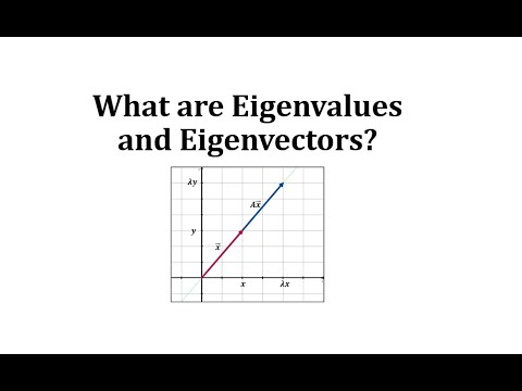
There is also a geometric significance to eigenvectors. When you have a nonzero vector which, when multiplied by a matrix results in another vector which is parallel to the first or equal to 0, this vector is called an eigenvector of the matrix. This is the meaning when the vectors are in $\mathbb{R}^{n}.$

The formal definition of eigenvalues and eigenvectors is as follows.

Definition $\PageIndex{1}$:Eigenvalues and Eigenvectors

Let $A$ be an $n\times n$ matrix and let $X \in \mathbb{C}^{n}$ be a nonzero vector for which

$$AX=\lambda X \label{eigen1}$$ for some scalar $\lambda .$ Then $\lambda$ is called an eigenvalue of the matrix $A$ and $X$ is called an eigenvector of $A$ associated with $\lambda$, or a $\lambda$-eigenvector of $A$.

The set of all eigenvalues of an $n\times n$ matrix $A$ is denoted by $\sigma \left( A\right)$ and is referred to as the spectrum of $A.$

The eigenvectors of a matrix $A$ are those vectors $X$ for which multiplication by $A$ results in a vector in the same direction or opposite direction to $X$. Since the zero vector $0$ has no direction this would make no sense for the zero vector. As noted above, $0$ is never allowed to be an eigenvector.

Let’s look at eigenvectors in more detail. Suppose $X$ satisfies $\eqref{eigen1}$. Then $$\begin{array}{c} AX - \lambda X = 0 \\ \mbox{or} \\ \left( A-\lambda I\right) X = 0 \end{array}\nonumber$$ for some $X \neq 0.$ Equivalently you could write $\left( \lambda I-A\right)X = 0$, which is more commonly used. Hence, when we are looking for eigenvectors, we are looking for nontrivial solutions to this homogeneous system of equations!

Recall that the solutions to a homogeneous system of equations consist of basic solutions, and the linear combinations of those basic solutions. In this context, we call the basic solutions of the equation $\left( \lambda I - A\right) X = 0$ basic eigenvectors. It follows that any (nonzero) linear combination of basic eigenvectors is again an eigenvector.

Suppose the matrix $\left(\lambda I - A\right)$ is invertible, so that $\left(\lambda I - A\right)^{-1}$ exists. Then the following equation would be true. $$\begin{aligned} X &= IX \\ &= \left( \left( \lambda I - A\right) ^{-1}\left(\lambda I - A \right) \right) X \\ &=\left( \lambda I - A\right) ^{-1}\left( \left( \lambda I - A\right) X\right) \\ &= \left( \lambda I - A\right) ^{-1}0 \\ &= 0\end{aligned}$$ This claims that $X=0$. However, we have required that $X \neq 0$. Therefore $\left(\lambda I - A\right)$ cannot have an inverse!

Recall that if a matrix is not invertible, then its determinant is equal to $0$. Therefore we can conclude that $$\det \left( \lambda I - A\right) =0 \label{eigen2}$$ Note that this is equivalent to $\det \left(A- \lambda I \right) =0$.

The expression $\det \left( \lambda I-A\right)$ is a polynomial (in the variable $x$) called the characteristic polynomial of $A$, and $\det \left( \lambda I-A\right) =0$ is called the characteristic equation. For this reason we may also refer to the eigenvalues of $A$ as characteristic values, but the former is often used for historical reasons.

Below is a video on eigenvalues and eigenvectors.

The following theorem claims that the roots of the characteristic polynomial are the eigenvalues of $A$. Thus when [eigen2] holds, $A$ has a nonzero eigenvector.

Theorem $\PageIndex{1}$: The Existence of an Eigenvector

Let $A$ be an $n\times n$ matrix and suppose $\det \left( \lambda I - A\right) =0$ for some $\lambda \in \mathbb{C}$.
Then $\lambda$ is an eigenvalue of $A$ and thus there exists a nonzero vector $X \in \mathbb{C}^{n}$ such that $AX=\lambda X$.

Proof

For $A$ an $n\times n$ matrix, the method of Laplace Expansion demonstrates that $\det \left( \lambda I - A \right)$ is a polynomial of degree $n.$ As such, the equation $\eqref{eigen2}$ has a solution $\lambda \in \mathbb{C}$ by the Fundamental Theorem of Algebra. The fact that $\lambda$ is an eigenvalue is left as an exercise.

Finding Eigenvectors and Eigenvalues

Now that eigenvalues and eigenvectors have been defined, we will study how to find them for a matrix $A$.

First, consider the following definition.

Definition $\PageIndex{2}$:Multiplicity of an Eigenvalue

Let $A$ be an $n \times n$ matrix with characteristic polynomial given by $\det \left( \lambda I - A\right)$. Then, the multiplicity of an eigenvalue $\lambda$ of $A$ is the number of times $\lambda$ occurs as a root of that characteristic polynomial.

For example, suppose the characteristic polynomial of $A$ is given by $\left( \lambda - 2 \right)^2$. Solving for the roots of this polynomial, we set $\left( \lambda - 2 \right)^2 = 0$ and solve for $\lambda$. We find that $\lambda = 2$ is a root that occurs twice. Hence, in this case, $\lambda = 2$ is an eigenvalue of $A$ of multiplicity equal to $2$.

Below is a video on finding $\lambda$ to make $A - \lambda I$ singular.

Below is a video on finding an eigenvalue from Ax=b.

We will now look at how to find the eigenvalues and eigenvectors for a matrix $A$ in detail. The steps used are summarized in the following procedure.

Procedure $\PageIndex{1}$:Finding Eigenvalues and Eigenvectors

Let $A$ be an $n \times n$ matrix.

1. First, find the eigenvalues $\lambda$ of $A$ by solving the equation $\det \left( \lambda I -A \right) = 0$.
2. For each $\lambda$, find the basic eigenvectors $X \neq 0$ by finding the basic solutions to $\left( \lambda I - A \right) X = 0$.

To verify your work, make sure that $AX=\lambda X$ for each $\lambda$ and associated eigenvector $X$.

We will explore these steps further in the following example.

Example $\PageIndex{2}$:Find the Eigenvalues and Eigenvectors

Let $A = \left[ \begin{array}{rr} -5 & 2 \\ -7 & 4 \end{array} \right]$. Find its eigenvalues and eigenvectors.

Solution

We will use Procedure $\PageIndex{1}$. First we find the eigenvalues of $A$ by solving the equation $$\det \left( \lambda I - A \right) =0\nonumber$$

This gives $$\begin{aligned} \det \left( \lambda \left[ \begin{array}{rr} 1 & 0 \\ 0 & 1 \end{array} \right] - \left[ \begin{array}{rr} -5 & 2 \\ -7 & 4 \end{array} \right] \right) &= 0 \\ \\ \det \left[ \begin{array}{cc} \lambda +5 & -2 \\ 7 & \lambda -4 \end{array} \right] &= 0 \end{aligned}$$

Computing the determinant as usual, the result is $$\lambda ^2 + \lambda - 6 = 0\nonumber$$

Solving this equation, we find that $\lambda_1 = 2$ and $\lambda_2 = -3$.

Now we need to find the basic eigenvectors for each $\lambda$. First we will find the eigenvectors for $\lambda_1 = 2$. We wish to find all vectors $X \neq 0$ such that $AX = 2X$. These are the solutions to $(2I - A)X = 0$. $$\begin{aligned} \left( 2 \left[ \begin{array}{rr} 1 & 0 \\ 0 & 1 \end{array}\right] - \left[ \begin{array}{rr} -5 & 2 \\ -7 & 4 \end{array}\right] \right) \left[ \begin{array}{c} x \\ y \end{array}\right] &= \left[ \begin{array}{r} 0 \\ 0 \end{array} \right] \\ \\ \left[ \begin{array}{rr} 7 & -2 \\ 7 & -2 \end{array}\right] \left[ \begin{array}{c} x \\ y \end{array}\right] &= \left[ \begin{array}{r} 0 \\ 0 \end{array} \right] \end{aligned}$$

The augmented matrix for this system and corresponding reduced row-echelon form are given by $$\left[ \begin{array}{rr|r} 7 & -2 & 0 \\ 7 & -2 & 0 \end{array}\right] \rightarrow \cdots \rightarrow \left[ \begin{array}{rr|r} 1 & -\frac{2}{7} & 0 \\ 0 & 0 & 0 \end{array} \right]\nonumber$$

The solution is any vector of the form $$\left[ \begin{array}{c} \frac{2}{7}s \\ s \end{array} \right] = s \left[ \begin{array}{r} \frac{2}{7} \\ 1 \end{array} \right]\nonumber$$

Multiplying this vector by $7$ we obtain a simpler description for the solution to this system, given by $$t \left[ \begin{array}{r} 2 \\ 7 \end{array} \right]\nonumber$$

This gives the basic eigenvector for $\lambda_1 = 2$ as $$\left[ \begin{array}{r} 2\\ 7 \end{array} \right]\nonumber$$

To check, we verify that $AX = 2X$ for this basic eigenvector.

$$\left[ \begin{array}{rr} -5 & 2 \\ -7 & 4 \end{array}\right] \left[ \begin{array}{r} 2 \\ 7 \end{array} \right] = \left[ \begin{array}{r} 4 \\ 14 \end{array}\right] = 2 \left[ \begin{array}{r} 2\\ 7 \end{array} \right]\nonumber$$

This is what we wanted, so we know this basic eigenvector is correct.

Next we will repeat this process to find the basic eigenvector for $\lambda_2 = -3$. We wish to find all vectors $X \neq 0$ such that $AX = -3X$. These are the solutions to $((-3)I-A)X = 0$. $$\begin{aligned} \left( (-3) \left[ \begin{array}{rr} 1 & 0 \\ 0 & 1 \end{array}\right] - \left[ \begin{array}{rr} -5 & 2 \\ -7 & 4 \end{array}\right] \right) \left[ \begin{array}{c} x \\ y \end{array}\right] &= \left[ \begin{array}{r} 0 \\ 0 \end{array} \right] \\ \left[ \begin{array}{rr} 2 & -2 \\ 7 & -7 \end{array}\right] \left[ \begin{array}{c} x \\ y \end{array}\right] &= \left[ \begin{array}{r} 0 \\ 0 \end{array} \right] \end{aligned}$$

The augmented matrix for this system and corresponding reduced row-echelon form are given by $$\left[ \begin{array}{rr|r} 2 & -2 & 0 \\ 7 & -7 & 0 \end{array}\right] \rightarrow \cdots \rightarrow \left[ \begin{array}{rr|r} 1 & -1 & 0 \\ 0 & 0 & 0 \end{array} \right]\nonumber$$

The solution is any vector of the form $$\left[ \begin{array}{c} s \\ s \end{array} \right] = s \left[ \begin{array}{r} 1 \\ 1 \end{array} \right]\nonumber$$

This gives the basic eigenvector for $\lambda_2 = -3$ as $$\left[ \begin{array}{r} 1\\ 1 \end{array} \right]\nonumber$$

To check, we verify that $AX = -3X$ for this basic eigenvector.

$$\left[ \begin{array}{rr} -5 & 2 \\ -7 & 4 \end{array}\right] \left[ \begin{array}{r} 1 \\ 1 \end{array} \right] = \left[ \begin{array}{r} -3 \\ -3 \end{array}\right] = -3 \left[ \begin{array}{r} 1\\ 1 \end{array} \right]\nonumber$$

This is what we wanted, so we know this basic eigenvector is correct.

Below is a video on finding eigenvalues of a matrix.

Below is a video on finding  eigenvectors given eigenvalues.

Below is a video on finding an eigenvalue given matrix A and an eigenvector.

The following is an example using Procedure $\PageIndex{1}$ for a $3 \times 3$ matrix.

Example $\PageIndex{3}$:Find the Eigenvalues and Eigencectors

Find the eigenvalues and eigenvectors for the matrix $$A=\left[ \begin{array}{rrr} 5 & -10 & -5 \\ 2 & 14 & 2 \\ -4 & -8 & 6 \end{array} \right]\nonumber$$

Solution

We will use Procedure $\PageIndex{1}$. First we need to find the eigenvalues of $A$. Recall that they are the solutions of the equation $$\det \left( \lambda I - A \right) =0\nonumber$$

In this case the equation is $$\det \left( \lambda \left[ \begin{array}{rrr} 1 & 0 & 0 \\ 0 & 1 & 0 \\ 0 & 0 & 1 \end{array} \right] - \left[ \begin{array}{rrr} 5 & -10 & -5 \\ 2 & 14 & 2 \\ -4 & -8 & 6 \end{array} \right] \right) =0\nonumber$$ which becomes $$\det \left[ \begin{array}{ccc} \lambda - 5 & 10 & 5 \\ -2 & \lambda - 14 & -2 \\ 4 & 8 & \lambda - 6 \end{array} \right] = 0\nonumber$$

Using Laplace Expansion, compute this determinant and simplify. The result is the following equation. $$\left( \lambda -5\right) \left( \lambda ^{2}-20\lambda +100\right) =0\nonumber$$

Solving this equation, we find that the eigenvalues are $\lambda_1 = 5, \lambda_2=10$ and $\lambda_3=10$. Notice that $10$ is a root of multiplicity two due to $$\lambda ^{2}-20\lambda +100=\left( \lambda -10\right) ^{2}\nonumber$$ Therefore, $\lambda_2 = 10$ is an eigenvalue of multiplicity two.

Now that we have found the eigenvalues for $A$, we can compute the eigenvectors.

First we will find the basic eigenvectors for $\lambda_1 =5.$ In other words, we want to find all non-zero vectors $X$ so that $AX = 5X$. This requires that we solve the equation $\left( 5 I - A \right) X = 0$ for $X$ as follows. $$\left( 5\left[ \begin{array}{rrr} 1 & 0 & 0 \\ 0 & 1 & 0 \\ 0 & 0 & 1 \end{array} \right] - \left[ \begin{array}{rrr} 5 & -10 & -5 \\ 2 & 14 & 2 \\ -4 & -8 & 6 \end{array} \right] \right) \left[ \begin{array}{r} x \\ y \\ z \end{array} \right] =\left[ \begin{array}{r} 0 \\ 0 \\ 0 \end{array} \right]\nonumber$$

That is you need to find the solution to $$\left[ \begin{array}{rrr} 0 & 10 & 5 \\ -2 & -9 & -2 \\ 4 & 8 & -1 \end{array} \right] \left[ \begin{array}{r} x \\ y \\ z \end{array} \right] =\left[ \begin{array}{r} 0 \\ 0 \\ 0 \end{array} \right]\nonumber$$

By now this is a familiar problem. You set up the augmented matrix and row reduce to get the solution. Thus the matrix you must row reduce is $$\left[ \begin{array}{rrr|r} 0 & 10 & 5 & 0 \\ -2 & -9 & -2 & 0 \\ 4 & 8 & -1 & 0 \end{array} \right]\nonumber$$ The reduced row-echelon form is $$\left[ \begin{array}{rrr|r} 1 & 0 & - \frac{5}{4} & 0 \\ 0 & 1 & \frac{1}{2} & 0 \\ 0 & 0 & 0 & 0 \end{array} \right]\nonumber$$ and so the solution is any vector of the form $$\left[ \begin{array}{c} \frac{5}{4}s \\ -\frac{1}{2}s \\ s \end{array} \right] =s\left[ \begin{array}{r} \frac{5}{4} \\ -\frac{1}{2} \\ 1 \end{array} \right]\nonumber$$ where $s\in \mathbb{R}$. If we multiply this vector by $4$, we obtain a simpler description for the solution to this system, as given by $$t \left[ \begin{array}{r} 5 \\ -2 \\ 4 \end{array} \right] \label{basiceigenvect}$$ where $t\in \mathbb{R}$. Here, the basic eigenvector is given by $$X_1 = \left[ \begin{array}{r} 5 \\ -2 \\ 4 \end{array} \right]\nonumber$$

Notice that we cannot let $t=0$ here, because this would result in the zero vector and eigenvectors are never equal to 0! Other than this value, every other choice of $t$ in $\eqref{basiceigenvect}$ results in an eigenvector.

It is a good idea to check your work! To do so, we will take the original matrix and multiply by the basic eigenvector $X_1$. We check to see if we get $5X_1$. $$\left[ \begin{array}{rrr} 5 & -10 & -5 \\ 2 & 14 & 2 \\ -4 & -8 & 6 \end{array} \right] \left[ \begin{array}{r} 5 \\ -2 \\ 4 \end{array} \right] = \left[ \begin{array}{r} 25 \\ -10 \\ 20 \end{array} \right] =5\left[ \begin{array}{r} 5 \\ -2 \\ 4 \end{array} \right]\nonumber$$ This is what we wanted, so we know that our calculations were correct.

Next we will find the basic eigenvectors for $\lambda_2, \lambda_3=10.$ These vectors are the basic solutions to the equation, $$\left( 10\left[ \begin{array}{rrr} 1 & 0 & 0 \\ 0 & 1 & 0 \\ 0 & 0 & 1 \end{array} \right] - \left[ \begin{array}{rrr} 5 & -10 & -5 \\ 2 & 14 & 2 \\ -4 & -8 & 6 \end{array} \right] \right) \left[ \begin{array}{r} x \\ y \\ z \end{array} \right] =\left[ \begin{array}{r} 0 \\ 0 \\ 0 \end{array} \right]\nonumber$$ That is you must find the solutions to $$\left[ \begin{array}{rrr} 5 & 10 & 5 \\ -2 & -4 & -2 \\ 4 & 8 & 4 \end{array} \right] \left[ \begin{array}{c} x \\ y \\ z \end{array} \right] =\left[ \begin{array}{r} 0 \\ 0 \\ 0 \end{array} \right]\nonumber$$

Consider the augmented matrix $$\left[ \begin{array}{rrr|r} 5 & 10 & 5 & 0 \\ -2 & -4 & -2 & 0 \\ 4 & 8 & 4 & 0 \end{array} \right]\nonumber$$ The reduced row-echelon form for this matrix is $$\left[ \begin{array}{rrr|r} 1 & 2 & 1 & 0 \\ 0 & 0 & 0 & 0 \\ 0 & 0 & 0 & 0 \end{array} \right]\nonumber$$ and so the eigenvectors are of the form $$\left[ \begin{array}{c} -2s-t \\ s \\ t \end{array} \right] =s\left[ \begin{array}{r} -2 \\ 1 \\ 0 \end{array} \right] +t\left[ \begin{array}{r} -1 \\ 0 \\ 1 \end{array} \right]\nonumber$$ Note that you can’t pick $t$ and $s$ both equal to zero because this would result in the zero vector and eigenvectors are never equal to zero.

Here, there are two basic eigenvectors, given by $$X_2 = \left[ \begin{array}{r} -2 \\ 1\\ 0 \end{array} \right] , X_3 = \left[ \begin{array}{r} -1 \\ 0 \\ 1 \end{array} \right]\nonumber$$

Taking any (nonzero) linear combination of $X_2$ and $X_3$ will also result in an eigenvector for the eigenvalue $\lambda =10.$ As in the case for $\lambda =5$, always check your work! For the first basic eigenvector, we can check $AX_2 = 10 X_2$ as follows. $$\left[ \begin{array}{rrr} 5 & -10 & -5 \\ 2 & 14 & 2 \\ -4 & -8 & 6 \end{array} \right] \left[ \begin{array}{r} -1 \\ 0 \\ 1 \end{array} \right] = \left[ \begin{array}{r} -10 \\ 0 \\ 10 \end{array} \right] =10\left[ \begin{array}{r} -1 \\ 0 \\ 1 \end{array} \right]\nonumber$$ This is what we wanted. Checking the second basic eigenvector, $X_3$, is left as an exercise.

Below is a video on finding the eigenvalues of a 3x3 matrix.

Below is a video on finding the eigenvalues of a 4x4 matrix.

It is important to remember that for any eigenvector $X$, $X \neq 0$. However, it is possible to have eigenvalues equal to zero. This is illustrated in the following example.

Example $\PageIndex{4}$:A Zero Eigenvalue

Let $$A=\left[ \begin{array}{rrr} 2 & 2 & -2 \\ 1 & 3 & -1 \\ -1 & 1 & 1 \end{array} \right]\nonumber$$ Find the eigenvalues and eigenvectors of $A$.

Solution

First we find the eigenvalues of $A$. We will do so using Definition $\PageIndex{1}$.

In order to find the eigenvalues of $A$, we solve the following equation. $$\det \left(\lambda I -A \right) = \det \left[ \begin{array}{ccc} \lambda -2 & -2 & 2 \\ -1 & \lambda - 3 & 1 \\ 1 & -1 & \lambda -1 \end{array} \right] =0\nonumber$$

This reduces to $\lambda ^{3}-6 \lambda ^{2}+8\lambda =0$. You can verify that the solutions are $\lambda_1 = 0, \lambda_2 = 2, \lambda_3 = 4$. Notice that while eigenvectors can never equal $0$, it is possible to have an eigenvalue equal to $0$.

Now we will find the basic eigenvectors. For $\lambda_1 =0$, we need to solve the equation $\left( 0 I - A \right) X = 0$. This equation becomes $-AX=0$, and so the augmented matrix for finding the solutions is given by $$\left[ \begin{array}{rrr|r} -2 & -2 & 2 & 0 \\ -1 & -3 & 1 & 0 \\ 1 & -1 & -1 & 0 \end{array} \right]\nonumber$$ The reduced row-echelon form is $$\left[ \begin{array}{rrr|r} 1 & 0 & -1 & 0 \\ 0 & 1 & 0 & 0 \\ 0 & 0 & 0 & 0 \end{array} \right]\nonumber$$ Therefore, the eigenvectors are of the form $t\left[ \begin{array}{r} 1 \\ 0 \\ 1 \end{array} \right]$ where $t\neq 0$ and the basic eigenvector is given by $$X_1 = \left[ \begin{array}{r} 1 \\ 0 \\ 1 \end{array} \right]\nonumber$$

We can verify that this eigenvector is correct by checking that the equation $AX_1 = 0 X_1$ holds. The product $AX_1$ is given by $$AX_1=\left[ \begin{array}{rrr} 2 & 2 & -2 \\ 1 & 3 & -1 \\ -1 & 1 & 1 \end{array} \right] \left[ \begin{array}{r} 1 \\ 0 \\ 1 \end{array} \right] = \left[ \begin{array}{r} 0 \\ 0 \\ 0 \end{array} \right]\nonumber$$

This clearly equals $0X_1$, so the equation holds. Hence, $AX_1 = 0X_1$ and so $0$ is an eigenvalue of $A$.

Computing the other basic eigenvectors is left as an exercise.

In the following sections, we examine ways to simplify this process of finding eigenvalues and eigenvectors by using properties of special types of matrices.

Eigenvalues and Eigenvectors for Special Types of Matrices

There are three special kinds of matrices which we can use to simplify the process of finding eigenvalues and eigenvectors. Throughout this section, we will discuss similar matrices, elementary matrices, as well as triangular matrices.

We begin with a definition.

Definition $\PageIndex{3}$:Similar Matrices

Let $A$ and $B$ be $n \times n$ matrices. Suppose there exists an invertible matrix $P$ such that $$A = P^{-1}BP\nonumber$$ Then $A$ and $B$ are called similar matrices.

It turns out that we can use the concept of similar matrices to help us find the eigenvalues of matrices. Consider the following lemma.

Lemma $\PageIndex{1}$:Similar Matrices and Eigenvalues

Let $A$ and $B$ be similar matrices, so that $A=P^{-1}BP$ where $A,B$ are $n\times n$ matrices and $P$ is invertible. Then $A,B$ have the same eigenvalues.

Proof

We need to show two things. First, we need to show that if $A=P^{-1}BP$, then $A$ and $B$ have the same eigenvalues. Secondly, we show that if $A$ and $B$ have the same eigenvalues, then $A=P^{-1}BP$.

Here is the proof of the first statement. Suppose $A = P^{-1}BP$ and $\lambda$ is an eigenvalue of $A$, that is $AX=\lambda X$ for some $X\neq 0.$ Then $$P^{-1}BPX=\lambda X\nonumber$$ and so $$BPX=\lambda PX\nonumber$$

Since $P$ is one to one and $X \neq 0$, it follows that $PX \neq 0$. Here, $PX$ plays the role of the eigenvector in this equation. Thus $\lambda$ is also an eigenvalue of $B$. One can similarly verify that any eigenvalue of $B$ is also an eigenvalue of $A$, and thus both matrices have the same eigenvalues as desired.

Proving the second statement is similar and is left as an exercise.

Note that this proof also demonstrates that the eigenvectors of $A$ and $B$ will (generally) be different. We see in the proof that $AX = \lambda X$, while $B \left(PX\right)=\lambda \left(PX\right)$. Therefore, for an eigenvalue $\lambda$, $A$ will have the eigenvector $X$ while $B$ will have the eigenvector $PX$.

The second special type of matrices we discuss in this section is elementary matrices. Recall from Definition 2.8.1 that an elementary matrix $E$ is obtained by applying one row operation to the identity matrix.

It is possible to use elementary matrices to simplify a matrix before searching for its eigenvalues and eigenvectors. This is illustrated in the following example.

Example $\PageIndex{5}$:Simplify Using Elementary Matrices

Find the eigenvalues for the matrix $$A = \left[ \begin{array}{rrr} 33 & 105 & 105 \\ 10 & 28 & 30 \\ -20 & -60 & -62 \end{array} \right]\nonumber$$

Solution

This matrix has big numbers and therefore we would like to simplify as much as possible before computing the eigenvalues.

We will do so using row operations. First, add $2$ times the second row to the third row. To do so, left multiply $A$ by $E \left(2,2\right)$. Then right multiply $A$ by the inverse of $E \left(2,2\right)$ as illustrated. $$\left[ \begin{array}{rrr} 1 & 0 & 0 \\ 0 & 1 & 0 \\ 0 & 2 & 1 \end{array} \right] \left[ \begin{array}{rrr} 33 & 105 & 105 \\ 10 & 28 & 30 \\ -20 & -60 & -62 \end{array} \right] \left[ \begin{array}{rrr} 1 & 0 & 0 \\ 0 & 1 & 0 \\ 0 & -2 & 1 \end{array} \right] =\left[ \begin{array}{rrr} 33 & -105 & 105 \\ 10 & -32 & 30 \\ 0 & 0 & -2 \end{array} \right]\nonumber$$ By Lemma $\PageIndex{1}$, the resulting matrix has the same eigenvalues as $A$ where here, the matrix $E \left(2,2\right)$ plays the role of $P$.

We do this step again, as follows. In this step, we use the elementary matrix obtained by adding $-3$ times the second row to the first row. $$\left[ \begin{array}{rrr} 1 & -3 & 0 \\ 0 & 1 & 0 \\ 0 & 0 & 1 \end{array} \right] \left[ \begin{array}{rrr} 33 & -105 & 105 \\ 10 & -32 & 30 \\ 0 & 0 & -2 \end{array} \right] \left[ \begin{array}{rrr} 1 & 3 & 0 \\ 0 & 1 & 0 \\ 0 & 0 & 1 \end{array} \right] =\left[ \begin{array}{rrr} 3 & 0 & 15 \\ 10 & -2 & 30 \\ 0 & 0 & -2 \end{array} \right] \label{elemeigenvalue}$$ Again by Lemma $\PageIndex{1}$, this resulting matrix has the same eigenvalues as $A$. At this point, we can easily find the eigenvalues. Let $$B = \left[ \begin{array}{rrr} 3 & 0 & 15 \\ 10 & -2 & 30 \\ 0 & 0 & -2 \end{array} \right]\nonumber$$ Then, we find the eigenvalues of $B$ (and therefore of $A$) by solving the equation $\det \left( \lambda I - B \right) = 0$. You should verify that this equation becomes $$\left(\lambda +2 \right) \left( \lambda +2 \right) \left( \lambda - 3 \right) =0\nonumber$$ Solving this equation results in eigenvalues of $\lambda_1 = -2, \lambda_2 = -2$, and $\lambda_3 = 3$. Therefore, these are also the eigenvalues of $A$.

Through using elementary matrices, we were able to create a matrix for which finding the eigenvalues was easier than for $A$. At this point, you could go back to the original matrix $A$ and solve $\left( \lambda I - A \right) X = 0$ to obtain the eigenvectors of $A$.

Notice that when you multiply on the right by an elementary matrix, you are doing the column operation defined by the elementary matrix. In $\eqref{elemeigenvalue}$ multiplication by the elementary matrix on the right merely involves taking three times the first column and adding to the second. Thus, without referring to the elementary matrices, the transition to the new matrix in $\eqref{elemeigenvalue}$ can be illustrated by $$\left[ \begin{array}{rrr} 33 & -105 & 105 \\ 10 & -32 & 30 \\ 0 & 0 & -2 \end{array} \right] \rightarrow \left[ \begin{array}{rrr} 3 & -9 & 15 \\ 10 & -32 & 30 \\ 0 & 0 & -2 \end{array} \right] \rightarrow \left[ \begin{array}{rrr} 3 & 0 & 15 \\ 10 & -2 & 30 \\ 0 & 0 & -2 \end{array} \right]\nonumber$$

The third special type of matrix we will consider in this section is the triangular matrix. Recall Definition 3.1.6 which states that an upper (lower) triangular matrix contains all zeros below (above) the main diagonal. Remember that finding the determinant of a triangular matrix is a simple procedure of taking the product of the entries on the main diagonal.. It turns out that there is also a simple way to find the eigenvalues of a triangular matrix.

In the next example we will demonstrate that the eigenvalues of a triangular matrix are the entries on the main diagonal.

Example $\PageIndex{6}$:Eigenvalues for a Triangular Matrix

Let $A=\left[ \begin{array}{rrr} 1 & 2 & 4 \\ 0 & 4 & 7 \\ 0 & 0 & 6 \end{array} \right] .$ Find the eigenvalues of $A$.

Solution

We need to solve the equation $\det \left( \lambda I - A \right) = 0$ as follows $$\begin{aligned} \det \left( \lambda I - A \right) = \det \left[ \begin{array}{ccc} \lambda -1 & -2 & -4 \\ 0 & \lambda -4 & -7 \\ 0 & 0 & \lambda -6 \end{array} \right] =\left( \lambda -1 \right) \left( \lambda -4 \right) \left( \lambda -6 \right) =0\end{aligned}$$

Solving the equation $\left( \lambda -1 \right) \left( \lambda -4 \right) \left( \lambda -6 \right) = 0$ for $\lambda$ results in the eigenvalues $\lambda_1 = 1, \lambda_2 = 4$ and $\lambda_3 = 6$. Thus the eigenvalues are the entries on the main diagonal of the original matrix.

The same result is true for lower triangular matrices. For any triangular matrix, the eigenvalues are equal to the entries on the main diagonal. To find the eigenvectors of a triangular matrix, we use the usual procedure.

In the next section, we explore an important process involving the eigenvalues and eigenvectors of a matrix.