When a differential equation is of the form , we can just integrate: . Unfortunately this method no longer works for the general form of the equation . Integrating both sides yields
Notice the dependence on in the integral.
Separable equations
Let us suppose that the equation is separable. That is, let us consider
for some functions and . Let us write the equation in the Leibniz notation
Then we rewrite the equation as
Now both sides look like something we can integrate. We obtain
If we can find closed form expressions for these two integrals, we can, perhaps, solve for
Example
Take the equation
First note that is a solution, so assume from now on, so that we can divide by . Write the equation as then
We compute the antiderivatives to get
Or
where is some constant. Because is a solution and because of the absolute value we actually can write:
for any number (including zero or negative).
We check:
Yay!
We should be a little bit more careful with this method. You may be worried that we were integrating in two different variables. We seemingly did a different operation to each side. Let us work through this method more rigorously. Take
We rewrite the equation as follows. Note that is a function of and so is
We integrate both sides with respect to
We use the change of variables formula (substitution) on the left hand side:
And we are done.
Implicit solutions
It is clear that we might sometimes get stuck even if we can do the integration. For example, take the separable equation
We separate variables,
We integrate to get
or perhaps the easier looking expression (where )
It is not easy to find the solution explicitly as it is hard to solve for . We, therefore, leave the solution in this form and call it an implicit solution. It is still easy to check that an implicit solution satisfies the differential equation. In this case, we differentiate with respect to , and remember that is a function of , to get
Multiply both sides by and divide by and you will get exactly the differential equation. We leave this computation to the reader.
If you have an implicit solution, and you want to compute values for , you might have to be tricky. You might get multiple solutions for each , so you have to pick one. Sometimes you can graph as a function of , and then flip your paper. Sometimes you have to do more.
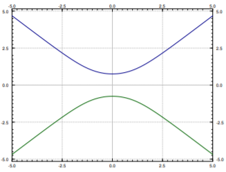
Computers are also good at some of these tricks. More advanced mathematical software usually has some way of plotting solutions to implicit equations. For example, for if you plot all the points that are solutions to , you find the two curves in Figure . This is not quite a graph of a function. For each there are two choices of . To find a function you would have to pick one of these two curves. You pick the one that satisfies your initial condition if you have one. For example, the top curve satisfies the condition . So for each we really got two solutions. As you can see, computing values from an implicit solution can be somewhat tricky. But sometimes, an implicit solution is the best we can do.
Figure : The implicit solution to .
The equation above also has the solution . So the general solution is These outlying solutions such as are sometimes called singular solutions.
Below is a video on solving a separable differential equation.
Example
Solve ,
Solution
First factor the right hand side to obtain
Separate variables, integrate, and solve for
Solve for the initial condition, to get (or , or , etc.). The particular solution we seek is, therefore,
Example
Juan made a cup of coffee, and Juan likes to drink coffee only once reaches 60 degrees Celsius and will not burn him. Initially at time minutes, Juan measured the temperature and the coffee was 89 degrees Celsius. One minute later, Juan measured the coffee again and it had 85 degrees. The temperature of the room (the ambient temperature) is 22 degrees. When should Juan start drinking?
Solution
Let be the temperature of the coffee in degrees Celsius, and let be the ambient (room) temperature, also in degrees Celsius. states that the rate at which the temperature of the coffee is changing is proportional to the difference between the ambient temperature and the temperature of the coffee. That is,
for some constant . For our setup , , . We separate variables and integrate (let and denote arbitrary constants)
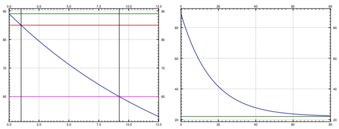
That is, . We plug in the first condition: , and hence . So . The second condition says . Solving for we get . Now we solve for the time that gives us a temperature of 60 degrees. Namely, we solve to get minutes. So Juan can begin to drink the coffee at just over 9 minutes from the time Juan made it. That is probably about the amount of time it took us to calculate how long it would take. See Figure .
Figure : Graphs of the coffee temperature function . On the left, horizontal lines are drawn at temperatures , , and . Vertical lines are drawn at and . Notice that the temperature of the coffee hits at , and at . On the right, the graph is over a longer period of time, with a horizontal line at the ambient temperature .
Example
Find the general solution to (including singular solutions).
Solution
First note that is a solution (a singular solution). Now assume that . So the general solution is,