
14.7: Variation of Parameters


- Last updated
- May 12, 2023
- Save as PDF

( \newcommand{\kernel}{\mathrm{null}\,}\)
In this section we give a method called variation of parameters for finding a particular solution of
P0(x)y″+P1(x)y′+P2(x)y=F(x)
if we know a fundamental set {y1,y2} of solutions of the complementary equation
P0(x)y″+P1(x)y′+P2(x)y=0.
Having found a particular solution yp by this method, we can write the general solution of Equation ??? as
y=yp+c1y1+c2y2.
Since we need only one nontrivial solution of Equation ??? to find the general solution of Equation ??? by reduction of order, it is natural to ask why we are interested in variation of parameters, which requires two linearly independent solutions of Equation ??? to achieve the same goal. Here’s the answer:
- If we already know two linearly independent solutions of Equation ??? then variation of parameters will probably be simpler than reduction of order.
- Variation of parameters generalizes naturally to a method for finding particular solutions of higher order linear equations (Section 9.4) and linear systems of equations (Section 10.7), while reduction of order doesn’t.
- Variation of parameters is a powerful theoretical tool used by researchers in differential equations. Although a detailed discussion of this is beyond the scope of this book, you can get an idea of what it means from Exercises 5.7.37–5.7.39.
We’ll now derive the method. As usual, we consider solutions of Equation ??? and Equation ??? on an interval (a,b) where P0, P1, P2, and F are continuous and P0 has no zeros. Suppose that {y1,y2} is a fundamental set of solutions of the complementary equation Equation ???. We look for a particular solution of Equation ??? in the form
yp=u1y1+u2y2
where u1 and u2 are functions to be determined so that yp satisfies Equation ???. You may not think this is a good idea, since there are now two unknown functions to be determined, rather than one. However, since u1 and u2 have to satisfy only one condition (that yp is a solution of Equation ???), we can impose a second condition that produces a convenient simplification, as follows.
Differentiating Equation ??? yields
y′p=u1y′1+u2y′2+u′1y1+u′2y2.
As our second condition on u1 and u2 we require that
u′1y1+u′2y2=0.
Then Equation ??? becomes
y′p=u1y′1+u2y′2;
that is, Equation ??? permits us to differentiate yp (once!) as if u1 and u2 are constants. Differentiating Equation ??? yields
y″p=u1y″1+u2y″2+u′1y′1+u′2y′2.
(There are no terms involving u″1 and u″2 here, as there would be if we hadn’t required Equation ???.) Substituting Equation ???, Equation ???, and Equation ??? into Equation ??? and collecting the coefficients of u1 and u2 yields
u1(P0y″1+P1y′1+P2y1)+u2(P0y″2+P1y′2+P2y2)+P0(u′1y′1+u′2y′2)=F.
As in the derivation of the method of reduction of order, the coefficients of u1 and u2 here are both zero because y1 and y2 satisfy the complementary equation. Hence, we can rewrite the last equation as
P0(u′1y′1+u′2y′2)=F.
Therefore yp in Equation ??? satisfies Equation ??? if
u′1y1+u′2y2=0u′1y′1+u′2y′2=FP0,
where the first equation is the same as Equation ??? and the second is from Equation ???.
We’ll now show that you can always solve Equation ??? for u′1 and u′2. (The method that we use here will always work, but simpler methods usually work when you’re dealing with specific equations.) To obtain u′1, multiply the first equation in Equation ??? by y′2 and the second equation by y2. This yields
u′1y1y′2+u′2y2y′2=0u′1y′1y2+u′2y′2y2=Fy2P0.
Subtracting the second equation from the first yields
u′1(y1y′2−y′1y2)=−Fy2P0.
Since {y1,y2} is a fundamental set of solutions of Equation ??? on (a,b), Theorem 5.1.6 implies that the Wronskian y1y′2−y′1y2 has no zeros on (a,b). Therefore we can solve Equation ??? for u′1, to obtain
u′1=−Fy2P0(y1y′2−y′1y2).
We leave it to you to start from Equation ??? and show by a similar argument that
u′2=Fy1P0(y1y′2−y′1y2).
We can now obtain u1 and u2 by integrating u′1 and u′2. The constants of integration can be taken to be zero, since any choice of u1 and u2 in Equation ??? will suffice.
You should not memorize Equation ??? and Equation ???. On the other hand, you don’t want to rederive the whole procedure for every specific problem. We recommend the a compromise:
- Write yp=u1y1+u2y2 to remind yourself of what you’re doing.
- Write the system u′1y1+u′2y2=0u′1y′1+u′2y′2=FP0 for the specific problem you’re trying to solve.
- Solve Equation ??? for u′1 and u′2 by any convenient method.
- Obtain u1 and u2 by integrating u′1 and u′2, taking the constants of integration to be zero.
- Substitute u1 and u2 into Equation ??? to obtain yp.
Below is a video on using variation of parameters to solve a differential equation.
Below is another video on using variation of parameters to solve a differential equation.
Find a particular solution yp of
x2y″−2xy′+2y=x9/2,
given that y1=x and y2=x2 are solutions of the complementary equation
x2y″−2xy′+2y=0.
Then find the general solution of Equation ???.
Solution
We set
yp=u1x+u2x2,
where
u′1x+2u′2x2=0u′1x+2u′2x2=x9/2x2=x5/2.
From the first equation, u′1=−u′2x. Substituting this into the second equation yields u′2x=x5/2, so u′2=x3/2 and therefore u′1=−u′2x=−x5/2. Integrating and taking the constants of integration to be zero yields
u1=−27x7/2andu2=25x5/2.
Therefore
yp=u1x+u2x2=−27x7/2x+25x5/2x2=435x9/2,
and the general solution of Equation ??? is
y=435x9/2+c1x+c2x2.
Below is a video on using variation of parameters to solve a differential equation.

Find a particular solution yp of
(x−1)y″−xy′+y=(x−1)2,
given that y1=x and y2=ex are solutions of the complementary equation
(x−1)y″−xy′+y=0.
Then find the general solution of Equation ???.
Solution
We set
yp=u1x+u2ex,
where
u′1x+u′2ex=0u′1x+u′2ex=(x−1)2x−1=x−1.
Subtracting the first equation from the second yields -u_1'(x-1)=x-1, so u_1'=-1. From this and the first equation, u_2'=-xe^{-x}u_1'=xe^{-x}. Integrating and taking the constants of integration to be zero yields
u_1=-x \quad \text{and} \quad u_2=-(x+1)e^{-x}. \nonumber
Therefore
y_p=u_1x+u_2e^x =(-x)x+(-(x+1)e^{-x})e^x=-x^2-x-1, \nonumber
so the general solution of Equation \ref{eq:5.7.16} is
\label{eq:5.7.17} y=y_p+c_1x+c_2e^x=-x^2-x-1+c_1x+c_2e^x = -x^2-1+(c_1-1)x+c_2e^x.
However, since c_1 is an arbitrary constant, so is c_1-1; therefore, we improve the appearance of this result by renaming the constant and writing the general solution as
\label{eq:5.7.18} y= -x^2-1+c_1x+c_2e^x.
There’s nothing wrong with leaving the general solution of Equation \ref{eq:5.7.16} in the form Equation \ref{eq:5.7.17}; however, we think you’ll agree that Equation \ref{eq:5.7.18} is preferable. We can also view the transition from Equation \ref{eq:5.7.17} to Equation \ref{eq:5.7.18} differently. In this example the particular solution y_p=-x^2-x-1 contained the term -x, which satisfies the complementary equation. We can drop this term and redefine y_p=-x^2-1, since -x^2-x-1 is a solution of Equation \ref{eq:5.7.16} and x is a solution of the complementary equation; hence, -x^2-1=(-x^2-x-1)+x is also a solution of Equation \ref{eq:5.7.16}. In general, it is always legitimate to drop linear combinations of \{y_1,y_2\} from particular solutions obtained by variation of parameters. (See Exercise 5.7.36 for a general discussion of this question.) We’ll do this in the following examples and in the answers to exercises that ask for a particular solution. Therefore, don’t be concerned if your answer to such an exercise differs from ours only by a solution of the complementary equation.
Below is a video on verifying a solution to a differential equation and then solving it using variation of parameters.
Find a particular solution of
\label{eq:5.7.19} y''+3y'+2y={1\over 1+e^x}.
Then find the general solution.
Solution
The characteristic polynomial of the complementary equation
\label{eq:5.7.20} y''+3y'+2y=0
is p(r)=r^2+3r+2=(r+1)(r+2), so y_1=e^{-x} and y_2=e^{-2x} form a fundamental set of solutions of Equation \ref{eq:5.7.20}. We look for a particular solution of Equation \ref{eq:5.7.19} in the form
y_p=u_1e^{-x}+u_2e^{-2x}, \nonumber
where
\begin{aligned} \phantom{-}u_1'e^{-x}+\phantom{2}u_2'e^{-2x}&=0\\ -u_1'e^{-x}-2u_2'e^{-2x}&={1\over 1+e^x}.\end{aligned}
Adding these two equations yields
-u_2'e^{-2x}={1\over1+e^x},\quad \text{so} \quad u_2'=-{e^{2x}\over 1+e^x}. \nonumber
From the first equation,
u_1'=-u_2'e^{-x}={e^x\over 1+e^x}. \nonumber
Integrating by means of the substitution v=e^x and taking the constants of integration to be zero yields
u_1=\int{e^x\over 1+e^x}\,dx=\int {dv\over 1+v} =\ln(1+v)=\ln(1+e^x) \nonumber
and
\begin{aligned} u_2&=-\int{e^{2x}\over 1+e^x}\,dx=-\int {v\over 1+v}\,dv =\int\left[{1\over 1+v}-1\right]\,dv \\ &=\ln(1+v)-v=\ln(1+e^x)-e^x.\end{aligned}
Therefore
\begin{aligned} y_p&=u_1e^{-x}+u_2e^{-2x}\\ &=[\ln(1+e^x)]e^{-x}+\left[\ln(1+e^x)-e^x\right]e^{-2x},\end{aligned}
so
y_p=\left(e^{-x}+e^{-2x}\right)\ln(1+e^x)-e^{-x}. \nonumber
Since the last term on the right satisfies the complementary equation, we drop it and redefine
y_p=\left(e^{-x}+e^{-2x}\right)\ln(1+e^x). \nonumber
The general solution of Equation \ref{eq:5.7.19} is
y=y_p+c_1e^{-x}+c_2e^{-2x}=\left(e^{-x}+e^{-2x}\right)\ln(1+e^x) +c_1e^{-x}+c_2e^{-2x}. \nonumber
Solve the initial value problem
\label{eq:5.7.21} (x^2-1)y''+4xy'+2y={2\over x+1}, \quad y(0)=-1,\quad y'(0)=-5,
given that
y_1={1\over x-1}\quad\mbox{ and }\quad y_2={1\over x+1} \nonumber
are solutions of the complementary equation
(x^2-1)y''+4xy'+2y=0. \nonumber
Solution
We first use variation of parameters to find a particular solution of
(x^2-1)y''+4xy'+2y={2\over x+1} \nonumber
on (-1,1) in the form
y_p={u_1\over x-1}+{u_2\over x+1}, \nonumber
where
\label{eq:5.7.22}\frac{u_{1}'}{x-1}+\frac{u_{2}'}{x+1}=0
-\frac{u_{1}'}{(x-1)^{2}}-\frac{u_{2}'}{(x+1)^{2}}=\frac{2}{(x+1)(x^{2}-1)}\nonumber
Multiplying the first equation by 1/(x-1) and adding the result to the second equation yields
\label{eq:5.7.23} \left[{1\over x^2-1}-{1\over(x+1)^2}\right]u_2'={2\over(x+1)(x^2-1)}.
Since
\left[{1\over x^2-1}-{1\over(x+1)^2}\right]={(x+1)-(x-1)\over(x+1)(x^2-1)} ={2\over(x+1)(x^2-1)}, \nonumber
Equation \ref{eq:5.7.23} implies that u_2'=1. From Equation \ref{eq:5.7.22},
u_1'=-{x-1\over x+1}u_2'=-{x-1\over x+1}. \nonumber
Integrating and taking the constants of integration to be zero yields
\begin{aligned} u_1&=-\int{x-1\over x+1}\,dx=-\int{x+1-2\over x+1}\,dx \\ &=\int\left[{2\over x+1}-1\right]\,dx=2\ln(x+1)-x\end{aligned}
and
u_2=\int\,dx=x. \nonumber
Therefore
\begin{aligned} y_p&={u_1\over x-1}+{u_2\over x+1}=\left[2\ln(x+1)-x\right]{1\over x-1} +x{1\over x+1} \\ &={2\ln(x+1)\over x-1}+x\left[{1\over x+1}-{1\over x-1}\right] ={2\ln(x+1)\over x-1}-{2x\over(x+1)(x-1)}.\end{aligned}
However, since
{2x\over(x+1)(x-1)}=\left[{1\over x+1}+{1\over x-1}\right] \nonumber
is a solution of the complementary equation, we redefine
y_p={2\ln(x+1)\over x-1}. \nonumber
Therefore the general solution of Equation \ref{eq:5.7.24} is
\label{eq:5.7.24} y={2\ln(x+1)\over x-1}+{c_1\over x-1}+{c_2\over x+1}.
Differentiating this yields
y'={2\over x^2-1}-{2\ln(x+1)\over(x-1)^2}-{c_1\over(x-1)^2}-{c_2\over(x+1)^2}. \nonumber
Setting x=0 in the last two equations and imposing the initial conditions y(0)=-1 and y'(0)=-5 yields the system
\begin{aligned} -c_1+c_2&=-1\phantom{.}\\ -2-c_1-c_2&=-5.\end{aligned}
The solution of this system is c_1=2,\,c_2=1. Substituting these into Equation \ref{eq:5.7.24} yields
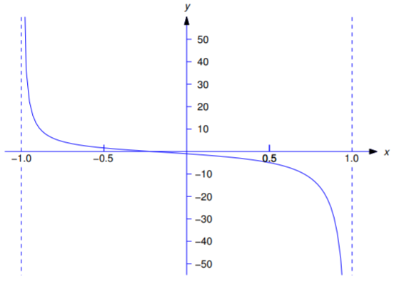
\begin{aligned} y&={2\ln(x+1)\over x-1}+{2\over x-1}+{1\over x+1}\\ &={2\ln(x+1)\over x-1}+{3x+1\over x^2-1}\end{aligned}
as the solution of Equation \ref{eq:5.7.21}. Figure 4.7.1 is a graph of the solution.
Below is a video on using variation of parameters to solve a differential equation.

We’ve now considered three methods for solving nonhomogeneous linear equations: undetermined coefficients, reduction of order, and variation of parameters. It’s natural to ask which method is best for a given problem. The method of undetermined coefficients should be used for constant coefficient equations with forcing functions that are linear combinations of polynomials multiplied by functions of the form e^{\alpha x}, e^{\lambda x}\cos \omega x, or e^{\lambda x}\sin \omega x. Although the other two methods can be used to solve such problems, they will be more difficult except in the most trivial cases, because of the integrations involved.
If the equation isn’t a constant coefficient equation or the forcing function isn’t of the form just specified, the method of undetermined coefficients does not apply and the choice is necessarily between the other two methods. The case could be made that reduction of order is better because it requires only one solution of the complementary equation while variation of parameters requires two. However, variation of parameters will probably be easier if you already know a fundamental set of solutions of the complementary equation.