16.1: Power Series

Many functions can be written in terms of a power series

$$\sum _{k=0}^{\infty} a_k(x-x_0)^k \nonumber$$

If we assume that a solution of a differential equation is written as a power series, then perhaps we can use a method reminiscent of undetermined coefficients. That is, we will try to solve for the numbers $a_k$. Before we can carry out this process, let us review some results and concepts about power series.

Definition

As we said, a power series is an expression such as

$$\label{eq:2} \sum_{k=0}^\infty a_k {(x-x_0)}^k =a_0 + a_1 (x-x_0) +a_2 {(x-x_0)}^2 +a_3 {(x-x_0)}^3 + \cdots ,$$

where $a_0,a_1,a_2,\ldots,a_k,\ldots$ and $x_0$ are constants. Let

$$S_n(x) = \sum_{k=0}^n a_k {(x-x_0)}^k =a_0 + a_1 (x-x_0) + a_2 {(x-x_0)}^2 + a_3 {(x-x_0)}^3 + \cdots + a_n {(x-x_0)}^n , \nonumber$$

denote the so-called partial sum. If for some $x$, the limit

$$\lim_{n\to \infty} S_n(x) = \lim_{n\to\infty} \sum_{k=0}^n a_k {(x-x_0)}^k \nonumber$$

exists, then we say that the series $\eqref{eq:2}$ converges at $x$. Note that for $x=x_0$, the series always converges to $a_0$. When $\eqref{eq:2}$ converges at any other point $x \neq x_0$, we say that $\eqref{eq:2}$ is a convergent power series. In this case we write

$$\sum_{k=0}^\infty a_k {(x-x_0)}^k = \lim_{n\to\infty} \sum_{k=0}^n a_k {(x-x_0)}^k. \nonumber$$

If the series does not converge for any point $x \neq x_0$, we say that the series is divergent.

Example $\PageIndex{1}$

The series

$$\sum_{k=0}^\infty \frac{1}{k!} x^k = 1 + x + \frac{x^2}{2} + \frac{x^3}{6} + \cdots \nonumber$$

is convergent for any $x$. Recall that $k! = 1\cdot 2\cdot 3 \cdots k$ is the factorial. By convention we define $0!=1$. In fact, you may recall that this series converges to $e^x$.

We say that $\eqref{eq:2}$ converges absolutely at $x$ whenever the limit

$$\lim_{n\to\infty} \sum_{k=0}^n \lvert a_k \rvert \, {\lvert x-x_0 \rvert}^k \nonumber$$

exists. That is, the series $\sum_{k=0}^\infty \lvert a_k \rvert \, {\lvert x-x_0 \rvert}^k$ is convergent. If $\eqref{eq:2}$ converges absolutely at $x$, then it converges at $x$. However, the opposite implication is not true.

Example $\PageIndex{2}$

The series

$$\sum_{k=1}^\infty \frac{1}{k} x^k \nonumber$$

converges absolutely for all $x$ in the interval $(-1,1)$.

It converges at $x=-1$, as

$\sum_{k=1}^\infty \frac{{(-1)}^k}{k}$ converges (conditionally)

by the alternating series test.

But the power series does not converge absolutely at $x=-1$, because $\sum_{k=1}^\infty \frac{1}{k}$ does not converge. The series diverges at $x=1$.

Radius of Convergence

If a power series converges absolutely at some $x_1$, then for all $x$ such that $\lvert x - x_0 \rvert \leq \lvert x_1 - x_0 \vert$ (that is, $x$ is closer than $x_1$ to $x_0$) we have $\bigl\lvert a_k {(x-x_0)}^k \bigr\rvert \leq \bigl\lvert a_k {(x_1-x_0)}^k \bigr\rvert$ for all $k$. As the numbers $\bigl\lvert a_k {(x_1-x_0)}^k \bigr\rvert$ sum to some finite limit, summing smaller positive numbers $\bigl\lvert a_k {(x-x_0)}^k \bigr\rvert$ must also have a finite limit. Hence, the series must converge absolutely at $x$.

Theorem $\PageIndex{1}$

For a power series $\eqref{eq:2}$, there exists a number $\rho$ (we allow $\rho =\infty$) called the radius of convergence such that the series converges absolutely on the interval $(x_{0}-\rho ,\:x_{0}+\rho )$ and diverges for $x<x_{0}-\rho$ and $x>x_{0}+\rho$. We write $\rho =\infty$ if the series converges for all $x$.

Figure $\PageIndex{1}$: Convergence of a power series.

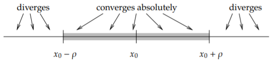
See Figure $\PageIndex{1}$. In Example $\PageIndex{1}$ the radius of convergence is $\rho = \infty$ as the series converges everywhere. In Example $\PageIndex{2}$ the radius of convergence is $\rho=1$. We note that $\rho = 0$ is another way of saying that the series is divergent. A useful test for convergence of a series is the ratio test. Suppose that

$$\sum_{k=0}^\infty c_k \nonumber$$

is a series such that the limit

$$L = \lim_{n\to\infty} \left \lvert \frac{c_{k+1}}{c_k} \right \rvert \nonumber$$

exists. Then the series converges absolutely if $L < 1$ and diverges if $L > 1$.

Let us apply this test to the series $\eqref{eq:2}$. That is we let $c_k = a_k {(x - x_0)}^k$ in the test. Compute

$$L = \lim_{n\to\infty} \left \lvert \frac{c_{k+1}}{c_k} \right \rvert = \lim_{n\to\infty} \left \lvert \frac{a_{k+1} {(x - x_0)}^{k+1}}{a_k {(x - x_0)}^k} \right \rvert = \lim_{n\to\infty} \left \lvert\frac{a_{k+1}}{a_k}\right \rvert \lvert x - x_0 \rvert . \nonumber$$

Define $A$ by

$$A =\lim_{n\to\infty} \left \lvert \frac{a_{k+1}}{a_k} \right \rvert . \nonumber$$

Then if $1 > L = A \lvert x - x_0 \rvert$ the series $\eqref{eq:2}$ converges absolutely. If $A = 0$, then the series always converges. If $A > 0$, then the series converges absolutely if $\lvert x - x_0 \rvert < \frac{1}{A}$, and diverges if $\lvert x - x_0 \rvert > \frac{1}{A}$. That is, the radius of convergence is $\frac{1}{A}$.

A similar test is the root test. Suppose

$$L=\lim_{k\to\infty} \sqrt[3]{|c_{k}|} \nonumber$$

exists. Then $\sum_{k=0}^{\infty}c_{k}$ converges absolutely if $L<1$ and diverges if $L>1$. We can use the same calculation as above to find $A$. Let us summarize.

Theorem $\PageIndex{2}$: Ratio and Root Tests for Power Series

Let

$$\sum_{k=0}^\infty a_k {(x-x_0)}^k \nonumber$$

be a power series such that

$$A = \lim_{n\to\infty} \left \lvert \frac{a_{k+1}}{a_k} \right \rvert\quad\text{or}\quad A=\lim_{k\to\infty}\sqrt[3]{|a_{k}|} \nonumber$$

exists. If $A = 0$, then the radius of convergence of the series is $\infty$. Otherwise the radius of convergence is $\frac{1}{A}$.

Below is a video on finding the interval of convergence of a power series.

Below is another video on finding the interval of convergence of a power series.

Example $\PageIndex{3}$

Suppose we have the series

$$\sum_{k=0}^\infty 2^{-k} {(x-1)}^k . \nonumber$$

First we compute,

$$A = \lim_{k\to\infty} \left \lvert \frac{a_{k+1}}{a_k} \right \rvert = \lim_{k\to\infty} \left \lvert \frac{2^{-k-1}}{2^{-k}} \right \rvert = 2^{-1} = \frac{1}{2}. \nonumber$$

Therefore the radius of convergence is $2$, and the series converges absolutely on the interval $(-1,3)$. And we could just as well have used the root test:

$$A = \lim_{k\to\infty} \lim_{k\to\infty} \sqrt[k]{\lvert a_k \rvert} = \lim_{k\to\infty} \sqrt[k]{\lvert 2^{-k} \rvert} = \lim_{k\to\infty} 2^{-1} = \frac{1}{2}. \nonumber$$

Below is a video on the interval of convergence of a power series not centered at the origin.

 

Example $\PageIndex{4}$

Consider $$\sum_{k=0}^\infty \frac{1}{k^k} {x}^k . \nonumber$$ Compute the limit for the root test, $$A = \lim_{k\to\infty} \sqrt[k]{\lvert a_k \rvert} = \lim_{k\to\infty} \sqrt[k]{ \left\lvert\frac{1}{k^k}\right\rvert} = \lim_{k\to\infty} \sqrt[k]{ {\left\lvert\frac{1}{k}\right\rvert}^{k}} = \lim_{k\to\infty} \frac{1}{k} = 0 . \nonumber$$ So the radius of convergence is $\infty$: the series converges everywhere. The ratio test would also work here.

The root or the ratio test does not always apply. That is the limit of $\bigl \lvert \frac{a_{k+1}}{a_k} \bigr \rvert$ or $\sqrt[k]{\lvert a_k \rvert}$ might not exist. There exist more sophisticated ways of finding the radius of convergence, but those would be beyond the scope of this chapter. The two methods above cover many of the series that arise in practice. Often if the root test applies, so does the ratio test, and vice versa, though the limit might be easier to compute in one way than the other.

Analytic Functions

Functions represented by power series are called analytic functions. Not every function is analytic, although the majority of the functions you have seen in calculus are. An analytic function $f(x)$ is equal to its Taylor series$^{1}$ near a point $x_0$. That is, for $x$ near $x_0$ we have

$$\label{eq:21} f(x) = \sum_{k=0}^\infty \frac{f^{(k)}(x_0)}{k!} {(x-x_0)}^k ,$$

where $f^{(k)}(x_0)$ denotes the $k^{\text{th}}$ derivative of $f(x)$ at the point $x_0$.

Figure $\PageIndex{2}$: The sine function and its Taylor approximations around $x_o=0$ of and degree.

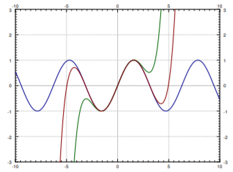
For example, sine is an analytic function and its Taylor series around $x_0 = 0$ is given by

$$\sin(x) = \sum_{n=0}^\infty \frac{{(-1)}^n}{(2n+1)!} x^{2n+1} . \nonumber$$

In Figure $\PageIndex{2}$ we plot $\sin(x)$ and the truncations of the series up to degree 5 and 9. You can see that the approximation is very good for $x$ near 0, but gets worse for $x$ further away from 0. This is what happens in general. To get a good approximation far away from $x_0$ you need to take more and more terms of the Taylor series.

Manipulating Power Series

One of the main properties of power series that we will use is that we can differentiate them term by term. That is, suppose that $\sum a_k {(x-x_0)}^k$ is a convergent power series. Then for $x$ in the radius of convergence we have

$$\frac{d}{dx} \left[\sum_{k=0}^\infty a_k {(x-x_0)}^k\right]=\sum_{k=1}^\infty k a_k {(x-x_0)}^{k-1} . \nonumber$$

Notice that the term corresponding to $k=0$ disappeared as it was constant. The radius of convergence of the differentiated series is the same as that of the original.

Example $\PageIndex{5}$

Let us show that the exponential $y=e^x$ solves $y'=y$. First write

$$y = e^x = \sum_{k=0}^\infty \frac{1}{k!} x^k . \nonumber$$

Now differentiate

$$y' = \sum_{k=1}^\infty k \frac{1}{k!} x^{k-1} =\sum_{k=1}^\infty \frac{1}{(k-1)!} x^{k-1} . \nonumber$$

We reindex the series by simply replacing $k$ with $k+1$. The series does not change, what changes is simply how we write it. After reindexing the series starts at $k=0$ again.

$$\sum_{k=1}^\infty \frac{1}{(k-1)!} x^{k-1} =\sum_{k+1=1}^\infty \frac{1}{\bigl((k+1)-1\bigr)!} x^{(k+1)-1} =\sum_{k=0}^\infty \frac{1}{k!} x^k . \nonumber$$

That was precisely the power series for $e^x$ that we started with, so we showed that $\frac{d}{dx} [ e^x ] = e^x$.

Convergent power series can be added and multiplied together, and multiplied by constants using the following rules. First, we can add series by adding term by term,

$$\left(\sum_{k=0}^\infty a_k {(x-x_0)}^k\right)+\left(\sum_{k=0}^\infty b_k {(x-x_0)}^k\right)=\sum_{k=0}^\infty (a_k+b_k) {(x-x_0)}^k . \nonumber$$

We can multiply by constants,

$$\alpha \left(\sum_{k=0}^\infty a_k {(x-x_0)}^k\right)=\sum_{k=0}^\infty \alpha a_k {(x-x_0)}^k . \nonumber$$

We can also multiply series together,

$$\left(\sum_{k=0}^\infty a_k {(x-x_0)}^k\right) \, \left(\sum_{k=0}^\infty b_k {(x-x_0)}^k\right)=\sum_{k=0}^\infty c_k {(x-x_0)}^k , \nonumber$$

where $c_k = a_0b_k + a_1 b_{k-1} + \cdots + a_k b_0$. The radius of convergence of the sum or the product is at least the minimum of the radii of convergence of the two series involved.

Below is a video on differentiation and integration using power series.

Power Series for Rational Functions

Polynomials are simply finite power series. That is, a polynomial is a power series where the $a_k$ are zero for all $k$ large enough. We can always expand a polynomial as a power series about any point $x_0$ by writing the polynomial as a polynomial in $(x-x_0)$. For example, let us write $2x^2-3x+4$ as a power series around $x_0 = 1$:

$$2x^2-3x+4 = 3 + (x-1) + 2{(x-1)}^2 . \nonumber$$

In other words $a_0 = 3$, $a_1 = 1$, $a_2 = 2$, and all other $a_k = 0$. To do this, we know that $a_k = 0$ for all $k \geq 3$ as the polynomial is of degree 2.

We write $a_0 + a_1(x-1) + a_2{(x-1)}^2$, we expand, and we solve for $a_0$, $a_1$, and $a_2$. We could have also differentiated at $x=1$and used the Taylor series formula $\eqref{eq:21}$.

Let us look at rational functions, that is, ratios of polynomials. An important fact is that a series for a function only defines the function on an interval even if the function is defined elsewhere. For example, for $-1 < x < 1$ we have

$$\frac{1}{1-x} = \sum_{k=0}^\infty x^k = 1 + x + x^2 + \cdots \nonumber$$

This series is called the geometric series. The ratio test tells us that the radius of convergence is $1$. The series diverges for $x \leq -1$ and $x \geq 1$, even though $\frac{1}{1-x}$ is defined for all $x \not= 1$.

We can use the geometric series together with rules for addition and multiplication of power series to expand rational functions around a point, as long as the denominator is not zero at $x_0$. Note that as for polynomials, we could equivalently use the Taylor series expansion $\eqref{eq:21}$.

Below is a video on finding a power series to represent a rational function.

Example $\PageIndex{5}$

Expand $\frac{x}{1+2x+x^2}$ as a power series around the origin ($x_0 = 0$) and find the radius of convergence. First, write $1+2x+x^2 = {(1+x)}^2 = {\bigl(1-(-x)\bigr)}^2$. Now we compute

$$\begin{align}\begin{aligned} \frac{x}{1+2x+x^2} &=x {\left( \frac{1}{1-(-x)} \right)}^2 \\ &=x { \left( \sum_{k=0}^{\infty} {(-1)}^k x^k \right)}^2 \\ &=x \left(\sum_{k=0}^{\infty} c_k x^k \right) \\ &= \sum_{k=0}^{\infty} c_k x^{k+1} ,\end{aligned}\end{align} \nonumber$$

where using the formula for the product of series we obtain, $c_0 = 1$, $c_1 = -1 -1 = -2$, $c_2 = 1+1+1 = 3$, etc $\ldots$.

Therefore

$$\frac{x}{1+2x+x^2}=\sum_{k=1}^\infty {(-1)}^{k+1} k x^k = x-2x^2+3x^3-4x^4+\cdots \nonumber$$

The radius of convergence is at least 1. We use the ratio test

$$\lim_{k\to\infty} \left\lvert \frac{a_{k+1}}{a_k} \right\rvert = \lim_{k\to\infty} \left\lvert \frac{{(-1)}^{k+2} (k+1)}{{(-1)}^{k+1}k} \right\rvert= \lim_{k\to\infty} \frac{k+1}{k}=1. \nonumber$$

So the radius of convergence is actually equal to 1.

When the rational function is more complicated, it is also possible to use method of partial fractions. For example, to find the Taylor series for $\frac{x^3+x}{x^2-1}$, we write

$$\frac{x^3+x}{x^2-1}=x + \frac{1}{1+x} - \frac{1}{1-x}=x + \sum_{k=0}^\infty {(-1)}^k x^k - \sum_{k=0}^\infty x^k= - x + \sum_{\substack{k=3 \\ k \text{ odd}}}^\infty (-2) x^k . \nonumber$$

Footnotes

[1] Named after the English mathematician Sir Brook Taylor (1685–1731).