5.4: Normal Distribution

Last updated
Save as PDF

Page ID: 50949

$ \newcommand{\vecs}[1]{\overset { \scriptstyle \rightharpoonup} {\mathbf{#1}} } $ $ \newcommand{\vecd}[1]{\overset{-\!-\!\rightharpoonup}{\vphantom{a}\smash {#1}}} $$\newcommand{\id}{\mathrm{id}}$ $ \newcommand{\Span}{\mathrm{span}}$ $ \newcommand{\kernel}{\mathrm{null}\,}$ $ \newcommand{\range}{\mathrm{range}\,}$ $ \newcommand{\RealPart}{\mathrm{Re}}$ $ \newcommand{\ImaginaryPart}{\mathrm{Im}}$ $ \newcommand{\Argument}{\mathrm{Arg}}$ $ \newcommand{\norm}[1]{\| #1 \|}$ $ \newcommand{\inner}[2]{\langle #1, #2 \rangle}$ $ \newcommand{\Span}{\mathrm{span}}$ $\newcommand{\id}{\mathrm{id}}$ $ \newcommand{\Span}{\mathrm{span}}$ $ \newcommand{\kernel}{\mathrm{null}\,}$ $ \newcommand{\range}{\mathrm{range}\,}$ $ \newcommand{\RealPart}{\mathrm{Re}}$ $ \newcommand{\ImaginaryPart}{\mathrm{Im}}$ $ \newcommand{\Argument}{\mathrm{Arg}}$ $ \newcommand{\norm}[1]{\| #1 \|}$ $ \newcommand{\inner}[2]{\langle #1, #2 \rangle}$ $ \newcommand{\Span}{\mathrm{span}}$$\newcommand{\AA}{\unicode[.8,0]{x212B}}$

In the previous sections you learned that sampling is an important tool for determining the characteristics of a population. Although the parameters of the population (mean, standard deviation, etc.) were unknown, random sampling was used to yield reliable estimates of these values. The estimates were plotted on graphs to provide a visual representation of the distribution of the sample mean for various sample sizes. It is now time to define some properties of the sampling distribution of the sample mean and to examine what we can conclude about the entire population based on it.

You have probably seen a "bell-shaped curve" before. It turns out that many data sets, particularly when the sample size is sufficiently large, are distributed symmetrically, with most data values around the center (mean) and few outliers, resulting in a bell-shaped curve. This is called a "normal distribution." For instance, the weights of all the people in a certain country are likely distributed normally, and so are their heights. Normal distributions can describe all sorts of data involving people's cholesterol level, blood pressure, duration of pregnancy, IQ (intelligence quotient) score, credit score, and many more. For instance, the pregnancy (gestation) period for humans is known to have an average of 266 days (38 weeks) with a standard deviation of 16 days. The average IQ score is defined as 100 with a standard deviation of 15. Your SAT and other standardized test scores are defined in similar ways.

But what does it mean, and how does this information help us?

When data values are distributed normally, given its mean and standard deviation, we can then standardize the normal distribution and calculate various percentages related to scores/values. For example, given that the IQ scores have a mean of 100 and a standard deviation of 15, one can conclude that only about 2.3% of the population have an IQ of 130 or higher.

Here is how this works. First, let us define the "Standard Normal Distribution."

Definition: Standard normal distribution

The standard normal distribution is the normal distribution (bell-shaped curve) with 0 as the mean and 1 as the standard deviation.

It turns out that there is a simple way to "convert" any normal distribution to the standard one. It involves what is known as the "$z$-score."

The $z$−score measures how many standard deviations a score is away from the mean. The $z$−score of a term x in a population distribution whose mean is $\mu $ and whose standard deviation $\sigma $ is given by:

\[z=\dfrac{x-\mu}{\sigma} \nonumber \]

Since $\sigma $ is always positive, $z$ will be positive when $x$ is greater than $\mu$ and negative when $x$ is less than $\mu $. A $z$−score of zero means that the term has the same value as the mean.

Example $\PageIndex{1}$

On a nationwide math test the mean was 65 and the standard deviation was 10. If Robert scored 81, what was his $z$−score?

Solution

\[\begin{array}{l}
z=\dfrac{x-\mu}{\sigma} \\
z=\dfrac{81-65}{10} \\
z=\dfrac{16}{10} \\
z=1.6
\end{array} \nonumber \]

This means Robert’s score was 1.6 standard deviations above the mean.

Example $\PageIndex{2}$

On a college entrance exam, the mean was 70 and the standard deviation was 8. If Helen’s $z$−score was −1.5, what was her exam mark?

Solution

\[\begin{array}{l}
z=\dfrac{x-\mu}{\sigma} \\
\therefore z \cdot \sigma=x-\mu \\
x=\mu+z \cdot \sigma \\
x=(70)+(-1.5)(8) \\
x=58
\end{array} \nonumber \]

Now you will see how $z$−scores are used to determine the probability of an event.

Table $\PageIndex{1}$
$z$-value	Probability (area)
0.00	0.0000
0.50	0.1915
1.00	0.3413
1.50	0.4332
2.00	0.4772
2.50	0.4938
3.00	0.4987 (almost 50%)

The graph above shows the standard normal distribution (with the mean 0). Each decimal number in the table represents the probability (percentage) that a data value is between 0 and the corresponding $z$-value. For instance, about 34% of all data values lie between $z$=0 (mean) and $z$=1.0. Using symmetry, then, we can conclude that about 68% (twice 34%) of all data values are within 1 standard deviation of the mean ($z$ between -1 and 1). The standard normal distribution has been extensively studied using advanced mathematics, and the probability can be calculated for any $z$-score. This table just shows a few of those numbers. It is known, for instance, that 99.74% of values lie within 3 standard deviations of the mean, and virtually everything is within 4 standard deviations of the mean.

Example $\PageIndex{3}$

Suppose that the cholesterol levels are normally distributed with a mean of 160 (mg/dl) with a standard deviation of 40 (mg/dl).

What is the $z$-score corresponding to the cholesterol level of 200 (mg/dl)? How about 260 (mg/dl)?
What percent of people have a cholesterol level between 160 and 200? How about 260 or higher?

Solution

Note that $\dfrac{200-160}{40}=1$, so the $z$-score for 200 (mg/dl) is 1.0. Similarly, $\dfrac{260-160}{40}=2.5$, so the $z$-score for 260 (mg/dl) is 2.5.
Between 160 and 200 would correspond to the z-score between 0 and 1. According to the table, this amounts to 0.3413, or about 34%. In other words, about 34% of all the people have a cholesterol level between 160 and 200. However, 260 mg/dl corresponds to $z$=2.5. The table shows that 49.38% of the people belong to the interval between $z$=0 and $z$=2.5. Adding the 50% of those who are below average ($z$ less than 0), this gives us 99.38% below $z$=2.5. Since 100-99.38=0.62 (%), only 0.62%, i.e., less than 1% of the population, has a cholesterol level 260 or higher. This person should go see the doctor immediately.

Example $\PageIndex{4}$

Suppose that IQ scores are distributed with a mean of 100 and a standard deviation of 15. What are the probabilities that one’s IQ score is

100 or above?
115 or above?
130 or above?
145 or above?

Solution

100 is the average, so by symmetry, exactly 50% of the population has an IQ score of 100 or better.
115 is one standard deviation above the mean, i.e., $z$ = 1.0. So, by the table, 34.13% of the population has an IQ score between 100 and 115. Since 50% is supposed to be above the average of 100 (by symmetry), this means 50 - 34.13 = 15.87 (%) has an IQ score above 115.
Similarly, 130 corresponds to $z$ = 2.0. The table has .4772, and 50 - 47.72 = 2.28 (%). In other words, less than 3 out of 100 people have an IQ score higher than 130.
Again, 145 corresponds to $z$ = 3.0, and the table shows .4987. 50-49.87=0.13 (%). This implies about 1 in 1000 has an IQ of 145 or higher.

It should be noted that various details of IQ testing have changed from time to time, and one’s IQ score also varies over time. Many controversies exist for IQ scores, and some even consider IQ scores unreliable. Interested readers can search for and find a lot of information on the Internet.

Exercises

A political scientist surveys 28 of the current 106 representatives in a state's congress. Of them, 14 said they were supporting a new education bill, 12 said there were not supporting the bill, and 2 were undecided.
1. What is the population of this survey?
2. What is the size of the population?
3. What is the size of the sample?
4. Give the sample statistic for the proportion of voters surveyed who said they were supporting the education bill.
5. Based on this sample, we might expect how many of the representatives to support the education bill?
The city of Raleigh has 9500 registered voters. There are two candidates for city council in an upcoming election: Brown and Feliz. The day before the election, a telephone poll of 350 randomly selected registered voters was conducted. 112 said they'd vote for Brown, 207 said they'd vote for Feliz, and 31 were undecided.
1. What is the population of this survey?
2. What is the size of the population?
3. What is the size of the sample?
4. Give the sample statistic for the proportion of voters surveyed who said they'd vote for Brown.
5. Based on this sample, we might expect how many of the 9500 voters to vote for Brown?
Identify the most relevant source of bias in this situation: A survey asks the following: Should the mall prohibit loud and annoying rock music in clothing stores catering to teenagers?
Identify the most relevant source of bias in this situation: To determine opinions on voter support for a downtown renovation project, a surveyor randomly questions people working in downtown businesses.
Identify the most relevant source of bias in this situation: A survey asks people to report their actual income and the income they reported on their IRS tax form.
Identify the most relevant source of bias in this situation: A survey randomly calls people from the phone book and asks them to answer a long series of questions.
Identify the most relevant source of bias in this situation: A survey asks the following: Should the death penalty be permitted if innocent people might die?
Identify the most relevant source of bias in this situation: A study seeks to investigate whether a new pain medication is safe to market to the public. They test by randomly selecting 300 men from a set of volunteers.
In a study, you ask the subjects their age in years. Is this data qualitative or quantitative?
In a study, you ask the subjects their gender. Is this data qualitative or quantitative?
Does this describe an observational study or an experiment: The temperature on randomly selected days throughout the year was measured.
Does this describe an observational study or an experiment? A group of students are told to listen to music while taking a test and their results are compared to a group not listening to music.
In a study, the sample is chosen by separating all cars by size, and selecting 10 of each size grouping. What is the sampling method?
In a study, the sample is chosen by writing everyone’s name on a playing card, shuffling the deck, then choosing the top 20 cards. What is the sampling method?
A team of researchers is testing the effectiveness of a new HPV vaccine. They randomly divide the subjects into two groups. Group 1 receives new HPV vaccine, and Group 2 receives the existing HPV vaccine. The patients in the study do not know which group they are in.
1. Which is the treatment group?
2. Which is the control group (if there is one)?
3. Is this study blind, double-blind, or neither?
4. Is this best described as an experiment, a controlled experiment, or a placebo controlled experiment?
For the clinical trials of a weight loss drug containing Garcinia cambogia the subjects were randomly divided into two groups. The first received an inert pill along with an exercise and diet plan, while the second received the test medicine along with the same exercise and diet plan. The patients do not know which group they are in, nor do the fitness and nutrition advisors.
1. Which is the treatment group?
2. Which is the control group (if there is one)?
3. Is this study blind, double-blind, or neither?
4. Is this best described as an experiment, a controlled experiment, or a placebo controlled experiment?
A teacher wishes to know whether the males in his/her class have more conservative attitudes than the females. A questionnaire is distributed assessing attitudes.
1. Is this a sampling or a census?
2. Is this an observational study or an experiment?
3. Are there any possible sources of bias in this study?
A study is conducted to determine whether people learn better with spaced or massed practice. Subjects volunteer from an introductory psychology class. At the beginning of the semester 12 subjects volunteer and are assigned to the massed-practice group. At the end of the semester 12 subjects volunteer and are assigned to the spaced-practice condition.
1. Is this a sampling or a census?
2. Is this an observational study or an experiment?
3. This study involves two kinds of non-random sampling: (1) Subjects are not randomly sampled from some specified population and (2) Subjects are not randomly assigned to groups. Which problem is more serious? What effect on the results does each have?
A farmer believes that playing Barry Manilow songs to his peas will increase their yield. Describe a controlled experiment the farmer could use to test his theory.
A sports psychologist believes that people are more likely to be extroverted as adults if they played team sports as children. Describe two possible studies to test this theory. Design one as an observational study and the other as an experiment. Which is more practical?
Studies are often done by pharmaceutical companies to determine the effectiveness of a treatment program. Suppose that a new AIDS antibody drug is currently under study. It is given to patients once the AIDS symptoms have revealed themselves. Of interest is the average length of time in months patients live once starting the treatment. Two researchers each follow a different set of 50 AIDS patients from the start of treatment until their deaths.
1. What is the population of this study?
2. List two reasons why the data may differ.
3. Can you tell if one researcher is correct and the other one is incorrect? Why?
4. Would you expect the data to be identical? Why or why not?
5. If the first researcher collected her data by randomly selecting 40 states, then selecting 1 person from each of those states. What sampling method is that?
6. If the second researcher collected his data by choosing 40 patients he knew. What sampling method would that researcher have used? What concerns would you have about this data set, based upon the data collection method?
Find a newspaper or magazine article, or the online equivalent, describing the results of a recent study (the results of a poll are not sufficient). Give a summary of the study’s findings, then analyze whether the article provided enough information to determine the validity of the conclusions. If not, produce a list of things that are missing from the article that would help you determine the validity of the study. Look for the things discussed in the text: population, sample, randomness, blind, control, placebos, etc.
The table below shows scores on a Math test.
1. Complete the frequency table for the Math test scores
2. Construct a histogram of the data
3. Construct a pie chart of the data

80	50	50	90	70	70	100	60	70	80	70	50
90	100	80	70	30	80	80	70	100	60	60	50

A group of adults where asked how many cars they had in their household
1. Complete the frequency table for the car number data
2. Construct a histogram of the data
3. Construct a pie chart of the data

1	4	2	2	1	2	3	3	1	4	2	2
1	2	1	3	2	2	1	2	1	1	1	2

A group of adults were asked how many children they have in their families. The bar graph to the right shows the number of adults who indicated each number of children.
1. How many adults where questioned?
2. What percentage of the adults questioned had 0 children?

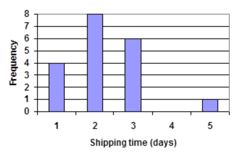
Jasmine was interested in how many days it would take an order from Netflix to arrive at her door. The graph below shows the data she collected.
1. How many movies did she order?
2. What percentage of the movies arrived in one day?

The bar graph below shows the percentage of students who received each letter grade on their last English paper. The class contains 20 students. What number of students earned an A on their paper?

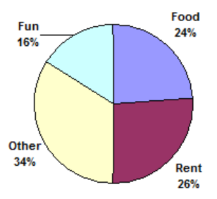
Kori categorized her spending for this month into four categories: Rent, Food, Fun, and Other. The percents she spent in each category are pictured here. If she spent a total of $2600 this month, how much did she spend on rent?

A group of diners were asked how much they would pay for a meal. Their responses were: $7.50, $8.25, $9.00, $8.00, $7.25, $7.50, $8.00, $7.00.
1. Find the mean
2. Find the median
3. Write the 5-number summary for this data
4. Find the standard deviation of this data
You recorded the time in seconds it took for 8 participants to solve a puzzle. The times were: 15.2, 18.8, 19.3, 19.7, 20.2, 21.8, 22.1, 29.4.
1. Find the mean
2. Find the median
3. Write the 5-number summary for this data
4. Find the standard deviation of this data
Refer back to the histogram from question #3.
1. Compute the mean number of children for the group surveyed
2. Compute the median number of children for the group surveyed
3. Write the 5-number summary for this data.
4. Create box plot.
Refer back to the histogram from question #4.
1. Compute the mean number of shipping days
2. Compute the median number of shipping days
3. Write the 5-number summary for this data.
4. Create box plot.
The box plot below shows salaries for Actuaries and CPAs. Kendra makes the median salary for an Actuary. Kelsey makes the first quartile salary for a CPA. Who makes more money? How much more?

Referring to the boxplot above, what percentage of actuaries makes more than the median salary of a CPA?

Exploration

35. Studies are often done by pharmaceutical companies to determine the effectiveness of a treatment program. Suppose that a new AIDS antibody drug is currently under study. It is given to patients once the AIDS symptoms have revealed themselves. Of interest is the average length of time in months patients live once starting the treatment. Two researchers each follow a different set of 40 AIDS patients from the start of treatment until their deaths. The following data (in months) are collected.

Researcher 1:

3; 4; 11; 15; 16; 17; 22; 44; 37; 16; 14; 24; 25; 15; 26; 27; 33; 29; 35; 44; 13; 21; 22; 10; 12; 8; 40; 32; 26; 27; 31; 34; 29; 17; 8; 24; 18; 47; 33; 34

Researcher 2:

3; 14; 11; 5; 16; 17; 28; 41; 31; 18; 14; 14; 26; 25; 21; 22; 31; 2; 35; 44; 23; 21; 21; 16; 12; 18; 41; 22; 16; 25; 33; 34; 29; 13; 18; 24; 23; 42; 33; 29

Create comparative histograms of the data
Create comparative boxplots of the data

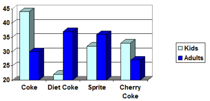
A graph appears below showing the number of adults and children who prefer each type of soda. There were 130 adults and kids surveyed. Discuss some ways in which the graph below could be improved.

Make up three data sets with 5 numbers each that have:
1. the same mean but different standard deviations.
2. the same mean but different medians.
3. the same median but different means.
A sample of 30 distance scores measured in yards has a mean of 7, a variance of 16, and a standard deviation of 4.
1. You want to convert all your distances from yards to feet, so you multiply each score in the sample by 3. What are the new mean, median, variance, and standard deviation?
2. You then decide that you only want to look at the distance past a certain point. Thus, after multiplying the original scores by 3, you decide to subtract 4 feet from each of the scores. Now what are the new mean, median, variance, and standard deviation?
Suppose that human pregnancies have an average duration of 270 days and standard deviation of 14 days. Find the probability that a pregnancy lasts for
1. Less than 270 days
2. Less than 263 days
3. More than 277 days
Suppose that in a youth basketball league, the average points for a team was 63 per game, with standard deviation 5. What is the probability that a team ends a game with
1. More than 68 points
2. Less than 53 points
3. More than 73 points
Suppose that the batting averages in baseball are normally distributed so that the mean is .258 and the standard deviation is 0.04. What is the probability that a player has a batting average of
1. More than .258?
2. More than .298?
3. More than .318?
In a certain country, people’s heights are normally distributed with a mean of 66 inches and a standard deviation of 3 inches. What is the probability that a person in that country is
1. Shorter than 60 inches?
2. Taller than 72 inches?
3. Shorter than 57 inches?

Reference

References (12)

Contributors and Attributions

Saburo Matsumoto
CC-BY-4.0