
6.1: Growth Models
- Page ID
- 50950
Populations of people, animals, and items are growing all around us. By understanding how things grow, we can better understand what to expect in the future. In this chapter, we focus on time-dependent change.
Linear Growth
Marco is a collector of antique soda bottles. His collection currently contains 437 bottles. Every year, he budgets enough money to buy 32 new bottles. Can we determine how many bottles he will have in 5 years, and how long it will take for his collection to reach 1000 bottles?
While both of these questions you could probably solve without an equation or formal mathematics, we are going to formalize our approach to this problem to provide a means to answer more complicated questions.
Suppose that \(P_n\) represents the number, or population, of bottles Marco has after \(n\) years. So \(P_0\) would represent the number of bottles now, \(P_1\) would represent the number of bottles after 1 year, \(P_2\) would represent the number of bottles after 2 years, and so on. We could describe how Marco’s bottle collection is changing using:
\[\begin{array}{l}
P_{0}=437 \\
P_{n}=P_{n-1}+32
\end{array} \nonumber \]
This is called a recursive relationship. A recursive relationship is a formula which relates the next value in a sequence to the previous values. Here, the number of bottles in year n can be found by adding 32 to the number of bottles in the previous year, \(P_{n-1}\). Using this relationship, we could calculate:
\[\begin{array}{l}
P_{1}=P_{0}+32=437+32=469 \\
P_{2}=P_{1}+32=469+32=501 \\
P_{3}=P_{2}+32=501+32=533 \\
P_{4}=P_{3}+32=533+32=565 \\
P_{5}=P_{4}+32=565+32=597
\end{array} \nonumber \]
We have answered the question of how many bottles Marco will have in 5 years. However, solving how long it will take for his collection to reach 1000 bottles would require a lot more calculations.
While recursive relationships are excellent for describing simply and cleanly how a quantity is changing, they are not convenient for making predictions or solving problems that stretch far into the future. For that, a closed or explicit form for the relationship is preferred. An explicit equation allows us to calculate \(P_n\) directly, without needing to know \(P_{n-1}\). While you may already be able to guess the explicit equation, let us derive it from the recursive formula. We can do so by selectively not simplifying as we go:
\[\begin{array}{ll}
P_{1}=437+32 & =437+1(32) \\
P_{2}=P_{1}+32=437+32+32 & =437+2(32) \\
P_{3}=P_{2}+32=(437+2(32))+32 & =437+3(32) \\
P_{4}=P_{3}+32=(437+3(32)) & =437+4(32)
\end{array} \nonumber \]
You can probably see the pattern now, and generalize that
\[P_{n}=437+n(32)=437+32 n \nonumber \]
Using this equation, we can calculate how many bottles he’ll have after 5 years:
\[P_{5}=437+32(5)=437+160=597 \nonumber \]
We can now also solve for when the collection will reach 1000 bottles by substituting in 1000 for \(P_n\) and solving for \(n\)
\[\begin{array}{l}
1000=437+32 n \\
563=32 n \\
n=563 / 32=17.59
\end{array} \nonumber \]
So Marco will reach 1000 bottles in 18 years.
In the previous example, Marco’s collection grew by the same number of bottles every year. This constant change is the defining characteristic of linear growth. Plotting the values we calculated for Marco’s collection, we can see the values form a straight line, the shape of linear growth.

Definition: Linear Growth
If a quantity starts at size \(P_0\) and grows by \(d\) every time period, then the quantity after \(n\) time periods can be determined as follows:
\[P_{n}=P_{0}+d \cdot n \nonumber \]
In this equation, \(d\) represents the common difference, the amount that the population changes each time \(n\) increases by 1.
Connection to prior learning: slope and intercept
You may recognize the common difference, \(d\), in our linear equation as slope. In fact, the entire explicit equation should look familiar – it is the same linear equation you learned in algebra, probably stated as \(y = mx + b\).
In the standard algebraic equation \(y = mx + b\), recall\(b\) was the y-intercept, or the \(y\) value when \(x\) was zero. In the form of the equation here, we are using \(P_0\) to represent that initial amount.
In the \(y = mx + b\) equation, recall that \(m\) was the slope. You might remember this as “rise over run” or the change in \(y\) divided by the change in \(x\). Either way, it represents the same thing as the common difference, \(d\), we are using, the amount the output \(P_n\) changes when the input \(n\) increases by 1.
The equations \(y = mx + b\) and \(P_{n}=P_{0}+d \cdot n\) mean the same thing and can be used the same ways. We’re just writing it somewhat differently.
Example \(\PageIndex{1}\)
The population of elk in a national forest was measured to be 12,000 in 2003 and was measured again to be 15,000 in 2007. If the population continues to grow linearly at this rate, what will the elk population be in 2014?
Solution
To begin, we need to define how we’re going to measure \(n\). Remember that \(P_0\) is the population when \(n = 0\), so we probably don’t want to literally use the year 0. Since we already know the population in 2003, let us define \(n = 0\) to be the year 2003. Then
\[P_0 = 12,000 \nonumber \]
Next we need to find \(d\). Remember \(d\) is the growth per time period, in this case growth per year. Between the two measurements, the population grew by 15,000-12,000 = 3,000, but it took 2007-2003 = 4 years to grow that much. To find the growth per year, we can divide: 3000 elk / 4 years = 750 elk in 1 year.
Alternatively, you can use the slope formula from algebra to determine the common difference, noting that the population is the output of the formula, and time is the input.
\[d=\text {slope}=\dfrac{15,000-12,000}{2007-2003}=\dfrac{3000}{4}=750 \nonumber \]
We can now write our equation.
\[P_{n}=12,000+750 n \nonumber \]
To answer the question, we need to first note that the year 2014 will be \(n = 11\), since 2014 is 11 years after 2003.
\[P_{11}=12,000+750(11)=20,250 \text { elk } \nonumber \]
Example \(\PageIndex{2}\)
Gasoline consumption in the US has been increasing steadily. Consumption data from 1992 to 2004 is shown below. Find a model for this data and use it to predict consumption in 2023. If the trend continues, when will consumption reach 200 billion gallons?
|
Year |
‘92 |
‘93 |
‘94 |
‘95 |
‘96 |
‘97 |
‘98 |
‘99 |
‘00 |
‘01 |
‘02 |
‘03 |
‘04 |
|---|---|---|---|---|---|---|---|---|---|---|---|---|---|
|
Consumption (billion of gallons) |
110 |
111 |
113 |
116 |
118 |
119 |
123 |
125 |
126 |
128 |
131 |
133 |
136 |
Solution
Plotting this data, it appears to have an approximately linear relationship:
While there are more advanced statistical techniques that can be used to find an equation to model the data, to get an idea of what is happening, we can find an equation by using two pieces of the data – perhaps the data from 1993 and 2003.

Letting \(n = 0\) correspond with 1993 would give \(P_0= 111\) billion gallons.
To find \(d\), we need to know how much the gas consumption increased each year, on average. From 1993 to 2003 the gas consumption increased from 111 billion gallons to 133 billion gallons, a total change of 133 – 111 = 22 billion gallons, over 10 years.
This gives us an average change of 22 billion gallons / 10 year = 2.2 billion gallons per year.
Equivalently,
\[d=\text {slope}=\dfrac{\text { change in output }}{\text { change in input }}=\dfrac{133-111}{10-0}=\dfrac{22}{10}=2.2 \text { billion gallons per year} \nonumber \]
\[P_{n}=111+2.2 n \nonumber \]
Calculating values using the explicit form and plotting them with the original data shows how well our model fits the data.

We can now use our model to make predictions about the future, assuming that the previous trend continues unchanged. To predict the gasoline consumption in 2023:
\(n\) = 30 (2023-1993=30 years later)
\(P_{23} = 111 + 2.2(30) = 177\)
Our model predicts that the US will consume 177 billion gallons of gasoline in 2023 if the current trend continues.
To find when the consumption will reach 200 billion gallons, we would set \(P_n = 200\), and solve for \(n\):
\[\begin{aligned} P_{n} &= 200 \quad \text { Replace } P_{n} \text { with our model} \\ 111+2.2 n &= 200 \quad \text { Subtract 111 from both sides} \\ 2.2 n &= 89 \quad \text { Divide both sides by } 2.2 \\ n &= 40.4545 \end{aligned} \nonumber \]
This tells us that consumption will reach 200 billion about 41 years after 1993, which would be in the year 2034.
By the way, the actual U.S. consumption in 2018 was 143 billion while this formula would give 166 billion. So, in reality, the growth rate appears to be going down a little.
Example \(\PageIndex{3}\)
The cost, in dollars, of a gym membership for \(n\) months can be described by the explicit equation \(P_n= 70 + 30n\). What does this equation tell us?
Solution
The value for \(P_0\) in this equation is 70, so the initial starting cost is $70. This tells us that there must be an initiation or start-up fee of $70 to join the gym.
The value for \(d\) in the equation is 30, so the cost increases by $30 each month. This tells us that the monthly membership fee for the gym is $30 a month. This is a pretty good deal.
Try it Now 1
The number of stay-at-home fathers in Canada has been growing steadily. While the trend is not perfectly linear, it is fairly linear. Use the data from 1976 and 2010 to find an explicit formula for the number of stay-at-home fathers; then use it to predict the number in 2020.
| Year | Number of stay-at-home fathers |
|---|---|
| 1976 | 20,610 |
| 1984 | 28,725 |
| 1991 | 43,530 |
| 2000 | 47,665 |
| 2010 | 53,555 |
When good models go bad
When using mathematical models to predict future behavior, it is important to keep in mind that very few trends will continue indefinitely.
Example \(\PageIndex{4}\)
Suppose a four-year old boy is currently 39 inches tall, and you are told to expect him to grow 2.5 inches a year. Setup a growth model.
Solution
We can set up a growth model, with \(n = 0\) corresponding to 4 years old.
\[P_n= 39 + 2.5n \nonumber \]
So at 6 years old, we would expect him to be
\(P_2= 39 + 2.5(2) = 44 \) inches tall
Most mathematical model will break down eventually. Certainly, we shouldn’t expect this boy to continue to grow at the same rate all his life. If he did, at age 50 he would be
\(P_{46}= 39 + 2.5(46) = 154\) inches tall = 12.8 feet tall!
Exponential Growth
Suppose that every year, only 10% of the fish in a lake have surviving offspring. Assuming that none of the adult fish dies, if there were 100 fish in the lake last year, there would now be 110 fish. If there were 1000 fish in the lake last year, there would now be 1100 fish. Absent of any inhibiting factors, populations of people and animals tend to grow by a percent of the existing population each year. Whenever a quantity grows by a fixed percentage rather than a fixed amount, the growth is exponential, like a compound interest.
Suppose our lake began with 1000 fish and 10% of the fish have surviving offspring each year. Since we start with 1000 fish, \(P_0 = 1000\). How do we calculate \(P_1\)? The new population will be the old population plus an additional 10%. Symbolically:
\[P_1=P_0+0.10P_0\]
Notice this could be condensed to a shorter form by factoring:
\[P_{1}=P_{0}+0.10 P_{0}=1 P_{0}+0.10 P_{0}=(1+0.10) P_{0}=1.10 P_{0}\]
While 10% is the growth rate, 1.10 is the growth multiplier. Notice that 1.10 can be thought of as “the original 100% plus an additional 10%”, which is 110% (of the original population).
For our fish population,
\[P_{0}=1.10(1000)=1100\]
We could then calculate the population in later years:
\[P_{2}=1.10 P_{1}=1.10(1100)=1210\]
\[P_{3}=1.10 P_{2}=1.10(1210)=1331\]
Notice that in the first year, the population grew by 100 fish, in the second year, the population grew by 110 fish, and in the third year the population grew by 121 fish. While there is a constant percentage growth, the actual increase in number of fish is increasing each year.
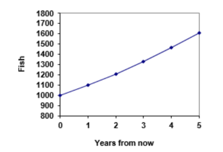
Graphing these values we see that this growth doesn’t quite appear linear.
To get a better picture of how this percentage-based growth affects things, we need an explicit form, so we can quickly calculate values further out in the future.
Like we did for the linear model, we will start building from the recursive equation:
\[\begin{array}{l}
P_{1}=1.10 P_{0}=1.10(1000) \\
P_{2}=1.10 P_{1}=1.10(1.10(1000))=1.10^{2}(1000) \\
P_{3}=1.10 P_{2}=1.10\left(1.10^{2}(1000)\right)=1.00^{3}(1000) \\
P_{4}=1.10 P_{3}=1.10\left(1.10^{3}(1000)\right)=1.10^{4}(1000)
\end{array} \nonumber \]
Observing a pattern, we can generalize the explicit form to be:
\(P_{n}=1.10^{n}(1000)\) or equivalently, \(P_{n}=1000\left(1.10^{n}\right)\). Note that this is exactly like the compound interest formula with \(r=10 \% \) annually.
From this, we can quickly calculate the number of fish in 10, 20, or 30 years:
\[\begin{array}{l}
P_{10}=1.10^{10}(1000)=2594 \\
P_{20}=1.10^{20}(1000)=6727 \\
P_{30}=1.10^{30}(1000)=17,449
\end{array} \nonumber \]
Adding these values to our graph reveals a shape that is definitely not linear. If our fish population had been growing linearly, by 100 fish each year, the population would have only reached 4000 in 30 years compared to almost 18,000 with this percent-based growth, called exponential growth.
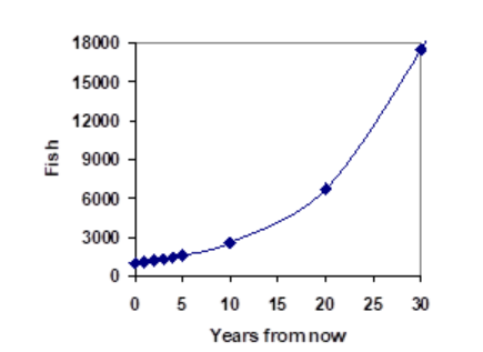
In exponential growth, the population grows proportional to the size of the population, so as the population gets larger, the same percent growth will yield a larger numeric growth.
Definition: Exponential Growth
If a quantity starts at size \(P_0\) and grows by \(R\%\) (written as a decimal, \(r\)) every time period, then the quantity after \(n\) time periods can be determined as follows:
\[P_{n}=P_{0}(1+r)^{n} \nonumber \]
We call \(r\) the growth rate.
Example \(\PageIndex{5}\)
Between 2007 and 2008, Olympia, WA grew almost 3% to a population of 245 thousand people. If this growth rate was to continue, what would the population of Olympia be in 2014?
Solution
As we did before, we first need to define what year will correspond to \(n = 0\). Since we know the population in 2008, it would make sense to have 2008 correspond to \(n = 0\), so \(P_0 = 245,000\). The year 2014 would then be \(n = 6\).
We know the growth rate is 3%, giving \(r = 0.03\).
Using the explicit form:
\[P_{6}=(1+0.03)^{6}(245,000)=1.19405(245,000)=292,542.25 \nonumber \]
The model predicts that in 2014, Olympia would have a population of about 293 thousand people.
Evaluating Exponents on the Calculator
To evaluate expressions like \((1.03)^6\), it will be easier to use a calculator than multiply 1.03 by itself six times. Most scientific calculators have a button for exponents. It is typically labeled:
\[^{\wedge}, \quad y^{x}, \text { or } \quad x^{y} \nonumber \]
To evaluate 1.036 we’d type 1.03 ^ 6, or 1.03 \(y^{x}\) 6.
Try it out. You should get an answer around 1.1940523.
Try it Now 2
India is the second most populous country in the world, with a population in 2008 of about 1.14 billion people. The population is growing by about 1.34% each year. If this trend continues, what will India’s population grow to by 2020?
Example \(\PageIndex{6}\)
A friend is using the equation \(P_n=4600(1.072)^n\) to predict the annual tuition at a local college. She says the formula is based on years after 2010. What does this equation tell us?
Solution
In the equation, \(P_0 = 4600\), which is the starting value of the tuition when \(n = 0\). This tells us that the tuition in 2010 was $4,600.
The growth multiplier is 1.072, so the growth rate is 0.072, or 7.2%. This tells us that the tuition is expected to grow by 7.2% each year.
Putting this together, we could say that the tuition in 2010 was $4,600 and is expected to grow by 7.2% each year.
Example \(\PageIndex{7}\)
In 1990, the residential energy use in the US was responsible for 962 million metric tons of carbon dioxide emissions. By the year 2000, that number had risen to 1182 million metric tons. If the emissions grow exponentially and continue at the same rate, what will the emissions grow to by 2050?
Solution
Similar to before, we will correspond \(n = 0\) with 1990, as that is the year for the first piece of data we have. That will make \(P_0 = 962\) (million metric tons of \(\ce{CO2}\)). In this problem, we are not given the growth rate, but instead are given that \(P_{10} = 1182}\).
When \(n = 10\), the explicit equation looks like:
\[P_{10}=(1+r)^{10} P_{0} \nonumber \]
We know the value for \(P_0\), so we can put that into the equation:
\[P_{10}=(1+r)^{10} 962 \nonumber \]
We also know that \(P_0 = 1182\), so substituting that in, we get
\[1182=(1+r)^{10} 962 \nonumber \]
We can now solve this equation for the growth rate, \(r\). Start by dividing by 962.
\[\begin{aligned} \dfrac{1182}{962} &= (1+r)^{10} \quad \text { Take the 10th root of both sides} \\ \sqrt[10]{\dfrac{1182}{962}} &= 1+r \quad \text { Subtract 1 from both sides} \\ r &= \sqrt[10]{\dfrac{1182}{962}}-1=0.0208=2.08 \% \end{aligned} \nonumber \]
So if the emissions are growing exponentially, they are growing by about 2.08% per year. We can now predict the emissions in 2050 by finding \(P_{60}\).
\(P_{60}=(1+0.0208)^{60} 962=3308.4\) million metric tons of \(\ce{CO2}\) in 2050 (That’s 3.3 billion metric tons!)
Rounding
As a note on rounding, notice that if we had rounded the growth rate to 2.1%, our calculation for the emissions in 2050 would have been 3347. Rounding to 2% would have changed our result to 3156. A very small difference in the growth rates gets magnified greatly in exponential growth. For this reason, it is recommended to round the growth rate as little as possible.
Evaluating Roots on the Calculator
In the previous example, we had to calculate the 10th root of a number. This is different from taking the basic square root, \(\sqrt{}\). Many scientific calculators have a button for general roots. It is typically labeled like
\[\sqrt[n]{}, \sqrt[x]{}, \text {or } \sqrt[y]{x} \nonumber \]
To evaluate the 3rd root of 8, for example, we’d either type \(3 \sqrt[x]{}\, 8\), or \(8 \sqrt[x]{}\, 3 \), depending on the calculator. Try it on yours to see which to use – you should get an answer of 2. If your calculator does not have a general root button, all is not lost. You can instead use the property of exponents which states that \(\sqrt[n]{a}=a^{1} / n\). So, to compute the 3rd root of 8, you could use your calculator’s exponent key to evaluate \(8^{1/3}\). To do this, type: \(8 y^{x}(1 \div 3)\) The parentheses tell the calculator to divide 1/3 before doing the exponent.
Try it Now 3
The number of users on a social networking site was 45 thousand in February when they officially went public and grew to 60 thousand by October. If the site is growing exponentially, and growth continues at the same rate, how many users should they expect two years after they went public?
Example \(\PageIndex{8}\)
Looking back at the last example, for the sake of comparison, what would the carbon emissions be in 2050 if emissions grow linearly at the same rate?
Solution
Again we will get \(n = 0\) correspond with 1990, giving \(P_0= 962\). To find d, we could take the same approach as earlier, noting that the emissions increased by 220 million metric tons in 10 years, giving a common difference of 22 million metric tons each year.
Alternatively, we could use an approach similar to that which we used to find the exponential equation. When \(n = 10\), the explicit linear equation looks like:
\[P_{10}=P_{0}+10 d \nonumber \]
We know the value for \(P_0\), so we can put that into the equation:
\[P_{10}=962+10 d \nonumber \]
Since we know that \(P_{10} = 1182\), substituting that in we get
\[1182=962+10 d \nonumber \]
We can now solve this equation for the common difference, d.
\[\begin{array}{l}
1182-962=10 d \\
220=10 d \\
d=22
\end{array} \nonumber \]
This tells us that if the emissions are changing linearly, they are growing by 22 million metric tons each year. Predicting the emissions in 2050,
\(P_{60}=962+22(60)=2282\) million metric tons.
You will notice that this number is substantially smaller than the prediction from the exponential growth model. Calculating and plotting more values helps illustrate the differences.

So how do we know which growth model to use when working with data? There are two approaches which should be used together whenever possible:
- Find more than two pieces of data. Plot the values, and look for a trend. Does the data appear to be changing like a line, or do the values appear to be curving upwards?
- Consider the factors contributing to the data. Are they things you would expect to change linearly or exponentially? For example, in the case of carbon emissions, we could expect that, absent other factors, they would be tied closely to population values, which tend to change exponentially.
Reference
- References (13)
Contributors and Attributions
Saburo Matsumoto
CC-BY-4.0