7.4: Fractals

Last updated
Save as PDF

Page ID: 50956

$ \newcommand{\vecs}[1]{\overset { \scriptstyle \rightharpoonup} {\mathbf{#1}} } $ $ \newcommand{\vecd}[1]{\overset{-\!-\!\rightharpoonup}{\vphantom{a}\smash {#1}}} $$\newcommand{\id}{\mathrm{id}}$ $ \newcommand{\Span}{\mathrm{span}}$ $ \newcommand{\kernel}{\mathrm{null}\,}$ $ \newcommand{\range}{\mathrm{range}\,}$ $ \newcommand{\RealPart}{\mathrm{Re}}$ $ \newcommand{\ImaginaryPart}{\mathrm{Im}}$ $ \newcommand{\Argument}{\mathrm{Arg}}$ $ \newcommand{\norm}[1]{\| #1 \|}$ $ \newcommand{\inner}[2]{\langle #1, #2 \rangle}$ $ \newcommand{\Span}{\mathrm{span}}$ $\newcommand{\id}{\mathrm{id}}$ $ \newcommand{\Span}{\mathrm{span}}$ $ \newcommand{\kernel}{\mathrm{null}\,}$ $ \newcommand{\range}{\mathrm{range}\,}$ $ \newcommand{\RealPart}{\mathrm{Re}}$ $ \newcommand{\ImaginaryPart}{\mathrm{Im}}$ $ \newcommand{\Argument}{\mathrm{Arg}}$ $ \newcommand{\norm}[1]{\| #1 \|}$ $ \newcommand{\inner}[2]{\langle #1, #2 \rangle}$ $ \newcommand{\Span}{\mathrm{span}}$$\newcommand{\AA}{\unicode[.8,0]{x212B}}$

Fractals are mathematical sets, usually obtained through recursion, that exhibit interesting dimensional properties. We’ll explore what that sentence means through the rest of this section. For now, we can begin with the idea of self-similarity, a characteristic of most fractals.

Definition: Self-similarity

A shape is self-similar when it looks essentially the same from a distance as it does closer up.

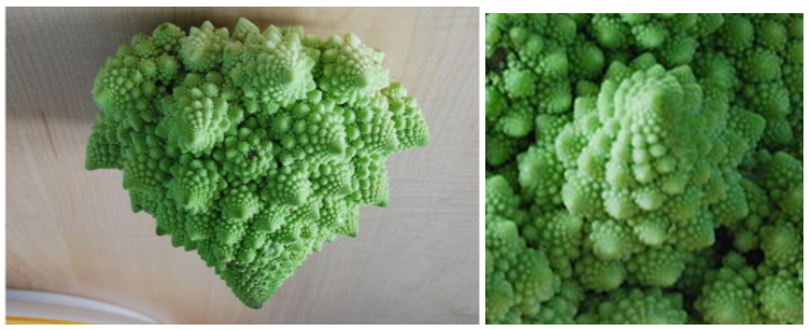
Self-similarity can often be found in nature. In the Romanesco broccoli pictured below, if we zoom in on part of the image, the piece remaining looks similar to the whole.

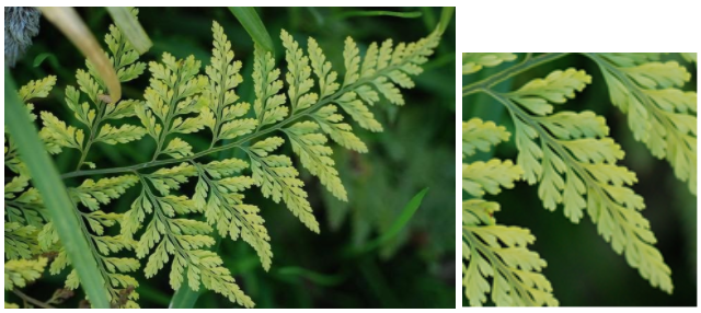
Figure $\PageIndex{1}$: Romanesco broccoli. (Image by AVM is licensed by CC 3.0)

Likewise, in the fern frond below, one piece of the frond looks similar to the whole.

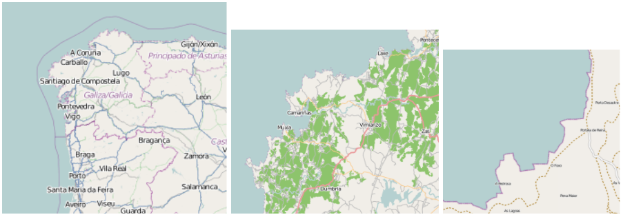
Figure $\PageIndex{2}$: Fern frond. (Image by Carolyn Jewel is licensed by CC 2.0)

Similarly, if we zoom in on the coastline of Portugal, each zoom reveals previously hidden detail, and the coastline, while not identical to the view from further way, does exhibit similar characteristics.

Figure $\PageIndex{3}$: Coastline of Portugal. (Image by OpenStreetMap is licensed by CC 3.0)

Iterated Fractals

This self-similar behavior can be replicated through recursion: repeating a process over and over.

Example $\PageIndex{1}$

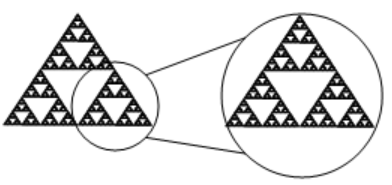
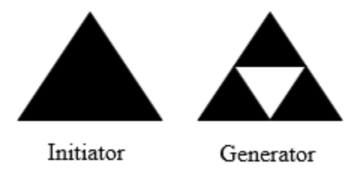
Suppose that we start with a filled-in triangle. We connect the midpoints of each side and remove the middle triangle. We then repeat this process.

Solution

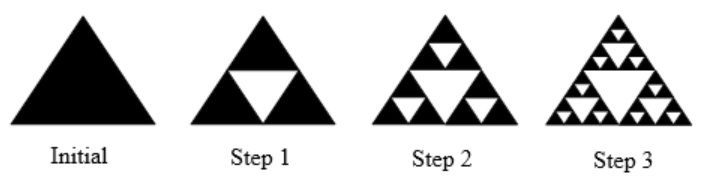
If we repeat this process, the shape that emerges is called the Sierpinski gasket. Notice that it exhibits self-similarity – any piece of the gasket will look identical to the whole. In fact, we can say that the Sierpinski gasket contains three copies of itself, each half as tall and wide as the original. Of course, each of those copies also contains three copies of itself.

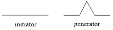
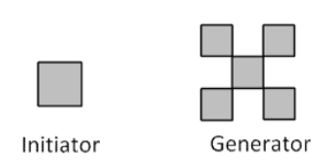
We can construct other fractals using a similar approach. To formalize this a bit, we’re going to introduce the idea of initiators and generators.

Definition: Initiators and Generators

An initiator is a starting shape.

A generator is an arranged collection of scaled copies of the initiator.

To generate fractals from initiators and generators, we follow a simple rule:

Fractal Generation Rule

At each step, replace every copy of the initiator with a scaled copy of the generator, rotating as necessary.

This process is easiest to understand through example.

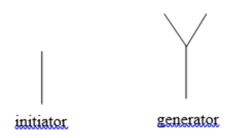
Example $\PageIndex{2}$

Use the initiator and generator shown to create the iterated fractal.

Solution

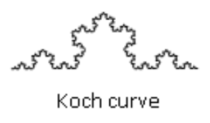
This tells us to, at each step, replace each line segment with the spiked shape shown in the generator. Notice that the generator itself is made up of 4 copies of the initiator. In step 1, the single line segment in the initiator is replaced with the generator. For step 2, each of the four line segments of step 1 is replaced with a scaled copy of the generator:

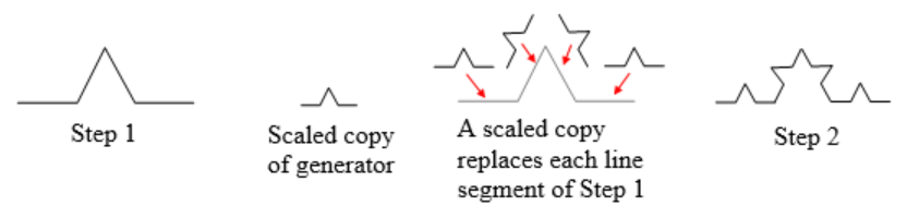
This process is repeated to form Step 3. Again, each line segment is replaced with a scaled copy of the generator.

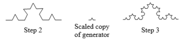
Notice that since Step 0 only had 1 line segment, Step 1 only required one copy of Step 0.

Since Step 1 had 4 line segments, Step 2 required 4 copies of the generator.

Step 2 then had 16 line segments, so Step 3 required 16 copies of the generator.

Step 4, then, would require 16*4 = 64 copies of the generator.

The shape resulting from iterating this process is called the Koch curve, named for Helge von Koch, who first explored it in 1904.

Notice that the Sierpinski gasket can also be described using the initiator-generator approach

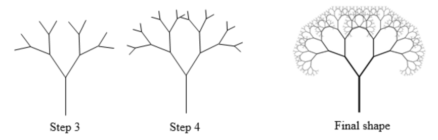
Figure $\PageIndex{10}$: Sierpinski gasket

Example $\PageIndex{3}$

Use the initiator and generator below; however, only iterate on the “branches.” Sketch several steps of the iteration.

Solution

We begin by replacing the initiator with the generator. We then replace each “branch” of Step 1 with a scaled copy of the generator to create Step 2.

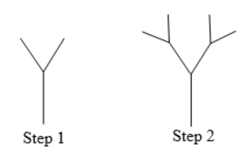
We can repeat this process to create later steps. Repeating this process can create intricate tree shapes.

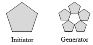
Figure $\PageIndex{13}$: Intricate tree shapes. (Image by Manuel Noah Angeja is licensed by CC 2.0)

Try it Now 1

Use the initiator and generator shown to produce the next two stages:

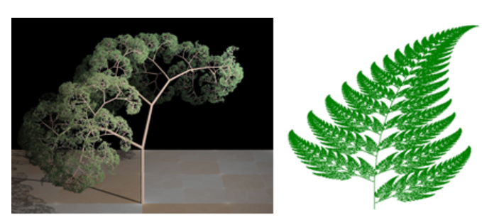
Using iteration processes like those above can create a variety of beautiful images evocative of nature.

Figure $\PageIndex{15}$: Image by Solkoll is in the public domain/Image by DSP-user is licensed by CC 3.0

More natural shapes can be created by adding in randomness to the steps.

Example $\PageIndex{4}$

Create a variation on the Sierpinski gasket by randomly skewing the corner points each time an iteration is made.

Solution

Suppose we start with the triangle below. We begin, as before, by removing the middle triangle. We then add in some randomness.

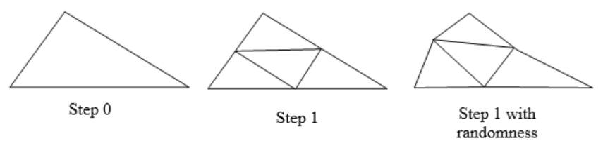
We then repeat this process.

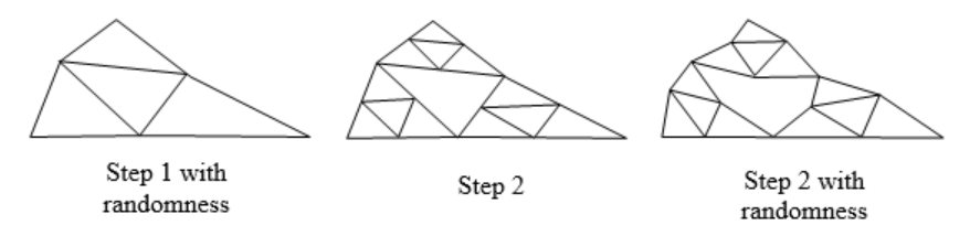
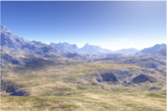
Continuing this process can create mountain-like structures.

The landscape below was created using fractals first and then colored and textured.

Figure $\PageIndex{18}$: Image by The Ostrich is licensed by CC 3.0

Fractal Dimension

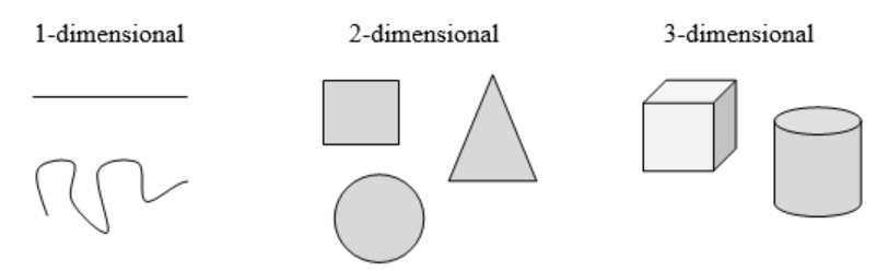
In addition to visual self-similarity, fractals exhibit other interesting properties. For example, notice that each step of the Sierpinski gasket iteration removes one quarter of the remaining area. If this process is continued indefinitely, we would end up essentially removing all the area, meaning we started with a 2-dimensional area and somehow end up with something less than that, but seemingly more than just a 1-dimensional line.

To explore this idea, we need to discuss dimension. Something like a line is 1-dimensional; it only has length. Any curve is 1-dimensional. Things like rectangles and circles are 2-dimensional since they have length and width, describing an area. Objects like boxes and cylinders have length, width, and height, describing a volume, and they are 3-dimensional.

Certain rules apply for scaling objects, and these rules are related to their dimension.

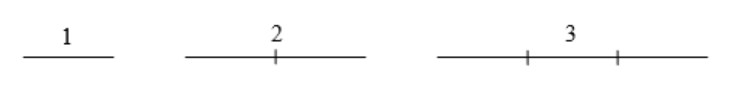
If I had a line with length 1 and wanted scale its length by 2, I would need two copies of the original line. If I had a line of length 1 and wanted to scale its length by 3, I would need three copies of the original.

If I had a rectangle with length 2 and height 1 and wanted to scale its length and width by 2, I would need four copies of the original rectangle. If I wanted to scale the length and width by 3, I would need nine copies of the original rectangle.

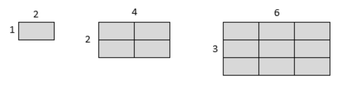
If I had a cubical box with sides of length 1 and wanted to scale its length, width, and height by 2, I would need eight copies of the original cube. If I wanted to scale the length, width and height by 3, I would need 27 copies of the original cube.

Notice that in the 1-dimensional case, copies needed = scale.

In the 2-dimensional case, copies needed = scale$^2$.

In the 3-dimensional case, copies needed = scale$^3$.

From these examples, we might infer a pattern.

In fact, in this section, we use this pattern to define the dimension of an object.

Scaling-Dimension Relation

To scale a D-dimensional shape by a scaling factor S, the number of copies C of the original shape needed will be given by:

\[\text {Copies } = \text { Scale }^{\text {Dimension }}, \text { or } C=S^{D} \nonumber \]

Example $\PageIndex{5}$

Use the scaling-dimension relation to determine the dimension of the Sierpinski gasket.

Solution

Suppose we define the original gasket to have side length 1. The larger gasket shown is twice as wide and twice as tall, so has been scaled by a factor of 2.

Notice that to construct the larger gasket, 3 copies of the original gasket are needed.

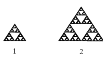
Using the scaling-dimension relation $C = S^D$, we obtain the equation $3 = 2^D$.

Since $2^1 = 2$ and $2^2 = 4$, we can immediately see that $D$ is somewhere between 1 and 2; the gasket is more than a 1-dimensional shape, but we’ve taken away so much area its now less than 2-dimensional.

Solving the equation $3 = 2^D$ requires logarithms. If you studied logarithms earlier, you may recall how to solve this equation (if not, just skip to the box below and use that formula):

\[\begin{aligned}
3 &= 2^{d} \quad \text {Take the logarithm of both sides}\\
\log (3) &= \log \left(2^{D}\right) \quad \text {Use the exponent property of } \log s\\
\log (3) &= D \log (2) \quad \text { Divide by } \log (2)\\
D &= \dfrac{\log (3)}{\log (2)} \approx 1.585
\end{aligned} \nonumber \]

The dimension of the gasket is about 1.585

Scaling-Dimension Relation, to find Dimension

To find the dimension $D$ of a fractal, determine the scaling factor $S$ and the number of copies $C$ of the original shape needed, then use the formula

\[D=\dfrac{\log (C)}{\log (S)} \nonumber \]

Try it Now 2

Use the initiator and generator shown to produce the next two stages.

We will now briefly mention another type of fractal, defined by a different type of recursion. To understand this type, you will need to know operations on complex numbers (including the imaginary number i), certain functions on those numbers, and iteration. These topics are beyond the scope of this text, so we will not include the details.

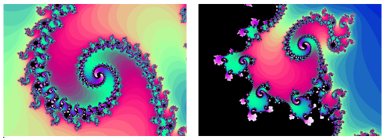
Here is what is known as the Mandelbrot set, defined using the iteration of a certain complex-valued function. Note that this well-known set, discovered in 1980, also shows a fractal-like shape. The boundary of this shape exhibits quasi-self-similarity, in that portions look very similar to the whole. In addition to coloring the Mandelbrot set itself black, it is common to the color the points in the complex plane surrounding the set.

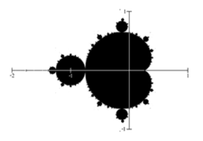
Figure $\PageIndex{25}$: Image by Connelly Barnes is in the public domain

Again, these colorings have specific mathematical meanings, but you will need to learn more advanced mathematics to fully appreciate the significance of these colors. All you need to know here is that these colors were not just added to make the pictures prettier. Studying some complex functions using certain colors resulted in these pretty pictures.

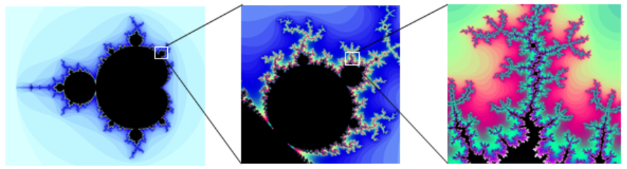
Figure $\PageIndex{26}$: Series created using Scott's Mandelbrot Set Explorer, licensed by CC 3.0

The Mandelbrot set, for having a simple definition, exhibits immense complexity. Zooming in on other portions of the set yields fascinating swirling shapes.

Figure $\PageIndex{27}$: Series created using Scott's Mandelbrot Set Explorer, licensed by CC 3.0

Additional Resources

The Mandelbrot Explorer site, provides more details on the Mandelbrot set, including a nice visualization of Mandelbrot sequences.

Exercises

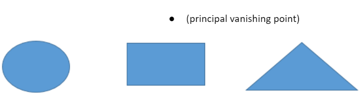
One side of a circular cylinder, a rectangular box, a triangular prism are shown below. Connect each vertex with the principal vanishing point to draw the cylinder, box, and prism.

Suppose you are sitting at the end of a long hallway, where the ceiling has rectangular panels ,the floor has square tiles, and the two side walls have vertical lines every few feet. Draw the hallway from your perspective, with a principal vanishing point. Now, what happens if you stand up? How would your picture change? How about if you move to the left?
Do some online research to find which artists seem to have used the Golden Ratio in their works of art. Give some examples of their art pieces.
Do some online research to find which composers seem to have written music that reflects the Golden Ratio. Give some specific examples of their music works.
Do some online research on the Golden Rectangle. Why is this called “golden”? Where do we see Golden Rectangles around us?
The Fibonacci Sequence begins with 1, 1, 2, 3, 5, 8, 13, 21, 34, 55, 89, … List the next three Fibonacci numbers (the next three terms of this sequence).
Do some online research on the Fibonacci Sequence. Find its relationship to the biological world, such as pine cones, sunflowers, nautilus shells, and human bodies.
Do some online research on the history of Fibonacci and his famous sequence. Who was he? What country is he from? Why did he study these numbers in particular?
A guitarist tunes his first (thinnest) string at E = 330 cps (typically denoted “E4”). If his sixth (thickest) string is to be two octaves lower, what is the frequency of the sixth string?
We started our musical scale at A4 = 440 cps. Some people may start a scale at C5 = 520 cps. Find the frequencies of the thirteen notes that spans an octave (C, C#, D, D#, E, F, F#, G, G#, A, A#, B, C), starting at C = 520 cps.
If A = 440 cps, the real “perfect fifth” would be E, whose frequency would be exactly 3/2 of A. What frequency is that? Compare that with the ‘tempered” frequency of E.
If A = 440 cps, the real “perfect fourth” would be D, whose frequency would be exactly 4/3 of A. What frequency is that? Compare that with the ‘tempered” frequency of D.
The range known as “tenor” is often defined from Second B (B2) to Third G (G3), about one and a half octave. Suppose that Middle C (C4) is 262 cps (and C3 is half of it), find the frequencies that cover this range. (Disclaimer: tenor opera singers have a much wider range than this. This is only the range normally referred to as “tenor.”)
It is said that Mariah Carey can hit a note as low as F2 and as high as G7 (slightly more than five octaves). Find the frequencies that cover this range. (Assume “A4” is 440 cps. A3 is half of it. A2 is half of that frequency. F2 is even lower. The numerical portion increases by 1 for each octave, and a new number starts with a C. So, for instance, the sequence goes like this: A2, A2#, B2, C3, C3#, …)

Using the initiator and generator shown, draw the next two stages of the iterated fractal.

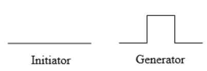
$clipboard_e402e84ba4fc079ea9b6038ec43f6c52a.png$
Figure $\PageIndex{29}$

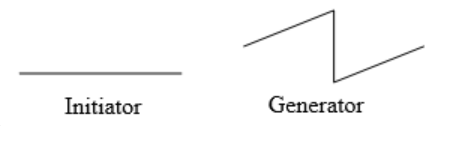
$clipboard_e399179e87f3b00d22c60330ae462289c.png$
Figure $\PageIndex{30}$
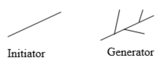
$clipboard_e36488474b9e91b191a9e7f5359ce8f9a.png$
Figure $\PageIndex{31}$
$clipboard_e37d06222729fce38b2dcbd4395b71844.png$
Figure $\PageIndex{32}$
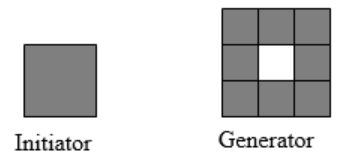
$clipboard_e1cc06e655bdbf95ac61ef8bf807ccd5e.png$
Figure $\PageIndex{33}$
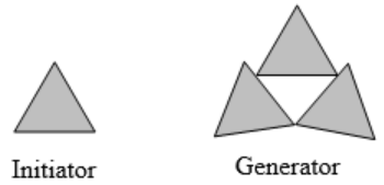
$clipboard_e0ddd2467ca75f87e396c98f93903ebe4.png$
Figure $\PageIndex{34}$
Create your own version of Sierpinski gasket with added randomness.
Create a version of the branching tree fractal from example #3 with added randomness.
Determine the fractal dimension of the Koch curve.
Determine the fractal dimension of the curve generated in exercise #1
Determine the fractal dimension of the Sierpinski carpet generated in exercise #5
Determine the fractal dimension of the Cantor set generated in exercise #4

Reference

References (18)

Contributors and Attributions

Saburo Matsumoto
CC-BY-4.0