7.1: Exponential Growth and Decay Models

Last updated
Save as PDF

Page ID: 40176

$ \newcommand{\vecs}[1]{\overset { \scriptstyle \rightharpoonup} {\mathbf{#1}} } $ $ \newcommand{\vecd}[1]{\overset{-\!-\!\rightharpoonup}{\vphantom{a}\smash {#1}}} $$\newcommand{\id}{\mathrm{id}}$ $ \newcommand{\Span}{\mathrm{span}}$ $ \newcommand{\kernel}{\mathrm{null}\,}$ $ \newcommand{\range}{\mathrm{range}\,}$ $ \newcommand{\RealPart}{\mathrm{Re}}$ $ \newcommand{\ImaginaryPart}{\mathrm{Im}}$ $ \newcommand{\Argument}{\mathrm{Arg}}$ $ \newcommand{\norm}[1]{\| #1 \|}$ $ \newcommand{\inner}[2]{\langle #1, #2 \rangle}$ $ \newcommand{\Span}{\mathrm{span}}$ $\newcommand{\id}{\mathrm{id}}$ $ \newcommand{\Span}{\mathrm{span}}$ $ \newcommand{\kernel}{\mathrm{null}\,}$ $ \newcommand{\range}{\mathrm{range}\,}$ $ \newcommand{\RealPart}{\mathrm{Re}}$ $ \newcommand{\ImaginaryPart}{\mathrm{Im}}$ $ \newcommand{\Argument}{\mathrm{Arg}}$ $ \newcommand{\norm}[1]{\| #1 \|}$ $ \newcommand{\inner}[2]{\langle #1, #2 \rangle}$ $ \newcommand{\Span}{\mathrm{span}}$$\newcommand{\AA}{\unicode[.8,0]{x212B}}$

Learning Objectives

In this section, you will learn to

Compare linear and exponential growth.
Recognize and model exponential growth and decay.

Prerequisite Skills

Before you get started, take this prerequisite quiz.

1. Simplify $3(2)^3$.

Click here to check your answer

$24$

If you missed this problem, review here and scroll to Example 4. (Note that this will open a different textbook in a new window.)

2. Simplify $-5(3)^2$.

Click here to check your answer

$-45$

If you missed this problem, review here and scroll to Example 4. (Note that this will open a different textbook in a new window.)

3. Solve $2^x=16$.

Click here to check your answer

$x=4$

If you missed this problem, review here. (Note that this will open a different textbook in a new window.)

4. Graph $y=-\dfrac{1}{2}x+3$.

Click here to check your answer

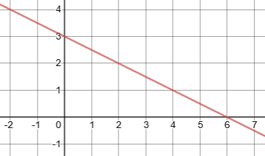
$clipboard_e1335126c95630ed2fbfdf2cc9347c448.png$

If you missed this problem, review Section 1.2. (Note that this will open in a new window.)

Comparing Exponential and Linear Growth

Consider two social media sites which are expanding the number of users they have:

Site A has 10,000 users, and expands by adding 1,500 new users each month
Site B has 10,000 users, and expands by increasing the number of users by 10% each month.

The number of users for Site A can be modeled as linear growth. The number of users increases by a constant number, 1500, each month. If $x$ = the number of months that have passed and $y$ is the number of users, the number of users after $x$ months is $y = 10000+1500x$. For site B, the user base expands by a constant percent each month, rather than by a constant number. Growth that occurs at a constant percent each unit of time is called exponential growth.

We can look at growth for each site to understand the difference. The table compares the number of users for each site for 12 months. The table shows the calculations for the first 4 months only, but uses the same calculation process to complete the rest of the 12 months.

Month	Users at Site A	Users at Site B
0	$10000$	$10000$
1	$10000 + 1500 = 11500$	$\begin{aligned} 10000+&10 \% \text { of } 10000 \\ =& 10000+0.10(10000) \\ =& 10000(1.10)=11000 \end{aligned}$
2	$11500 + 1500 = 13000$	$\begin{aligned} 11000+&10 \% \text { of } 11000 & \\ =&11000+0.10(11000) \\ =&11000(1.10)=12100 \end{aligned}$
3	$13000 + 1500 = 14500$	$\begin{aligned} 12100+&10 \% \text { of } 12100 & \\ =&12100+0.10(12100) \\ =&12100(1.10)=13310 \end{aligned}$
4	$14500 + 1500 = 16000$	$\begin{aligned} 13310+&10 \% \text { of } 13310 \\ =&13310+0.10(13310) \\ =&13310(1.10)=14641 \end{aligned}$
5	$17500$	$16105$
6	$19000$	$17716$
7	$20500$	$19487$
8	$22000$	$21436$
9	$23500$	$23579$
10	$25000$	$25937$
11	$26500$	$28531$
12	$28000$	$31384$

For Site B, we can re-express the calculations to help us observe the patterns and develop a formula for the number of users after x months.

Month 1: $y = 10000(1.1) = 11000$
Month 2: $y = 11000(1.1) = 10000(1.1)(1.1)=\mathbf{10000(1.1)^2}= 12100$
Month 3: $y = 12100(1.1) = 10000(1.1)^2 (1.1)=\mathbf{10000(1.1)^3}= 13310$
Month 4: $y = 13310(1.1) = 10000(1.1)^3 (1.1)=\mathbf{10000(1.1)^4}= 14641$

By looking at the patterns in the calculations for months 2, 3, and 4, we can generalize the formula. After $x$ months, the number of users $y$ is given by the function $\mathbf{y = 10000(1.1)^x}$

Example $\PageIndex{1}$

Determine whether each of the following statements represent exponential growth or linear growth.

The population of a certain town has been increasing by 2.4% over each of the last 10 years.
The population of a certain town has been increasing by 1,000 people over each of the last 10 years.
The number of bacterial cells increases by a factor of $\dfrac{3}{2}$ every 24 hours.

Solution

a. Since the population has been increasing by a constant percent for each unit of time, this is an example of exponential growth.

b. Since the population has been increasing by a constant number for each unit of time, this is an example of linear growth.

c. Since the number of cells has been increasing by a constant percent $ (\dfrac{3}{2}=150\%) $ for each unit of time, this is an example of exponential growth.

Using Exponential Functions to Model Growth and Decay

In exponential growth, the value of the dependent variable $y$ increases at a constant percentage rate as the value of the independent variable ($x$ or $t$) increases. Examples of exponential growth functions include:

the number of residents of a city or nation that grows at a constant percent rate.
the amount of money in a bank account that earns interest if money is deposited at a single point in time and left in the bank to compound without any withdrawals.

In exponential decay, the value of the dependent variable y decreases at a constant percentage rate as the value of the independent variable ($x$ or $t$) increases. Examples of exponential decay functions include:

value of a car or equipment that depreciates at a constant percent rate over time
the amount a drug that still remains in the body as time passes after it is ingested
the amount of radioactive material remaining over time as a radioactive substance decays.

Exponential functions often model quantities as a function of time; thus we often use the letter $t$ as the independent variable instead of $x$.

The table compares exponential growth and exponential decay functions:

Exponential Growth	Exponential Decay
Quantity grows by a constant percent per unit of time	Quantity decreases by a constant percent per unit of time
\(\mathbf{y=ab^x}\) \(a\) is a positive number representing the initial value of the function when \(x = 0\) \(b\) is a real number that is greater than 1: \(b > 1\) the growth rate \(r\) is a positive number, \(r > 0\) where \(b = 1+ r\) (so that \(r = b-1\))	\(\mathbf{y=ab^x}\) \(a\) is a positive number representing the initial value of the function when \(x = 0\) \(b\) is a real number that is between 0 and 1: \(0 < b < 1\) the decay rate \(r\) is a negative number, \(r < 0\) where \(b = 1+ r\) (so that \(r = b-1\))

Exponential Growth

Exponential Decay

Quantity grows by a constant percent
per unit of time

Quantity decreases by a constant percent per unit of time

$\mathbf{y=ab^x}$

$a$ is a positive number representing the initial value of the function when $x = 0$
$b$ is a real number that is greater than 1: $b > 1$
the growth rate $r$ is a positive number, $r > 0$ where $b = 1+ r$ (so that $r = b-1$)

$\mathbf{y=ab^x}$

$a$ is a positive number representing the initial value of the function when $x = 0$
$b$ is a real number that is between 0 and 1: $0 < b < 1$
the decay rate $r$ is a negative number, $r < 0$ where $b = 1+ r$ (so that $r = b-1$)

In general, the domain of exponential functions is the set of all real numbers. The range of an exponential growth or decay function is the set of all positive real numbers.

In most applications, the independent variable, $x$ or $t$, represents time. When the independent variable represents time, we may choose to restrict the domain so that independent variable can have only non-negative values in order for the application to make sense. If we restrict the domain, then the range is also restricted as well.

For an exponential growth function $y=ab^x$ with $b>1$ and $a > 0$, if we restrict the domain so that $x ≥ 0$, then the range is $y ≥ a$.
For an exponential decay function $y=ab^x$ with $0<b<1$ and $a > 0$, if we restrict the domain so that $x ≥ 0$, then the range is $0 < y ≤ a$.

Example $\PageIndex{2}$

Consider the growth models for social media sites A and B, where $x$ = number of months since the site was started and $y$ = number of users. The number of users for Site A follows the linear growth model:

\[y = 10000+1500x \nonumber.\]

The number of users for Site B follows the exponential growth model:

\[y=10000(1.1^x) \nonumber\]

For each site, use the function to calculate the number of users at the end of the first year, to verify the values in the table. Then use the functions to predict the number of users after 30 months.

Solution

Since $x$ is measured in months, then $x = 12$ at the end of one year.

Linear Growth Model:

When $x = 12$ months, then $y = 10000 + 1500(12) = 28,000$ users
When $x = 30$ months, then $y = 10000 + 1500(30) = 55,000$ users

Exponential Growth Model:

When $x = 12$ months, then $y = 10000(1.1^{12}) = 31,384$ users
When $x = 30$ months, then $y = 10000(1.1^{30}) =174,494$ users

We see that as $x$, the number of months, gets larger, the exponential growth function grows large faster than the linear function (even though in Example $\PageIndex{2}$ the linear function initially grew faster). This is an important characteristic of exponential growth: exponential growth functions always grow faster and larger in the long run than linear growth functions.

It is helpful to use function notation, writing $y = f(t) = ab^t$, to specify the value of $t$ at which the function is evaluated.

Example $\PageIndex{3}$

A forest has a population of 2000 squirrels that is increasing at the rate of 3% per year. Let $t$ = number of years and $y = f(t) =$ number of squirrels at time $t$.

Find the exponential growth function that models the number of squirrels in the forest at the end of $t$ years.
Use the function to find the number of squirrels after 5 years and after 10 years

Solution

a. The exponential growth function is $y = f(t) = ab^t$, where $a = 2000$ because the initial population is 2000 squirrels

The annual growth rate is 3% per year, stated in the problem. We will express this in decimal form as $r = 0.03$

Then $b = 1+r = 1+0.03 = 1.03$

Answer: The exponential growth function is $y = f(t) = 2000(1.03)^t$

b. After 5 years, the squirrel population is $y = f(5) = 2000(1.03)^5 \approx 2319$ squirrels

After 10 years, the squirrel population is $y = f(10) = 2000(1.03)^{10} \approx 2688$ squirrels

Example $\PageIndex{4}$

A large lake has a population of 1000 frogs. Unfortunately the frog population is decreasing at the rate of 5% per year. Let $t$ = number of years and $y$ = $g(t)$ = the number of frogs in the lake at time $t$.

Find the exponential decay function that models the population of frogs.
Calculate the size of the frog population after 10 years.

Solution

a. The exponential decay function is $y = g(t) = ab^t$, where $a = 1000$ because the initial population is 1000 frogs

The annual decay rate is 5% per year, stated in the problem. The words decrease and decay indicated that $r$ is negative. We express this as $r = -0.05$ in decimal form.

Then, $b = 1+ r = 1+ (-0.05) = 0.95$

Answer: The exponential decay function is: $y = g(t) = 1000(0.95)^t$

b. After 10 years, the frog population is $y = g(10) = 1000(0.95)^{10} \approx 599$ frogs

Example $\PageIndex{5}$

A population of bacteria is given by the function $y = f(t) = 100(2)^t$, where $t$ is time measured in hours and $y$ is the number of bacteria in the population.

What is the initial population?
What happens to the population in the first hour?
How long does it take for the population to reach 800 bacteria?

Solution

a. The initial population is 100 bacteria. We know this because $a = 100$ and because at time $t = 0$, then $f(0) = 100(2)^0 = 100(1)=100$

b. At the end of 1 hour, the population is $y = f(1) = 100(2)^1 = 100(2)=200$ bacteria.
The population has doubled during the first hour.

c. We need to find the time $t$ at which $f(t) = 800$. Substitute 800 as the value of $y$:

\[\begin{array}{l}
y=f(t)=100\left(2\right)^{t} \\
800=100\left(2\right)^{t}
\end{array}\nonumber\]

Divide both sides by 100 to isolate the exponential expression on the one side

\[8=1\left(2\right)^{\mathrm{t}} \nonumber\]

8 = 2³, so it takes $t = 3$ hours for the population to reach 800 bacteria.

Two important notes about Example $\PageIndex{5}$:

In solving $8 = 2^t$, we “knew” that $t$ is 3. But we usually can not know the value of the variable just by looking at the equation. Later we will use logarithms to solve equations that have the variable in the exponent.
To solve $800 = 100(2)^t$, we divided both sides by 100 to isolate the exponential expression $2^t$. We can not multiply 100 by 2. The exponent applies only to the quantity immediately before it, so the exponent t applies only to the base of 2.

Comparing Linear, Exponential and Polynomial Functions

To identify the type of function from its formula, we need to carefully note the position that the variable occupies in the formula.

A linear function can be written in the form $\mathbf{y=a x+b}$

As we studied in chapter 1, there are other forms in which linear equations can be written, but linear functions can all be rearranged to have form $y = mx + b$.

An exponential function has form $\mathbf{y=ab^x}$

The variable $\mathbf{x}$ is in the exponent. The base $b$ is a positive number.

If $b>1$, the function represents exponential growth.
If $0 < b < 1$, the function represents exponential decay

A polynomial function has form $\mathbf{y=ax^P+bx^{P-1}+cx^{P-2}+...}$

The variable $\mathbf{x}$ is in the base. The exponent $p$ is a non-zero number, and the exponents decrease until the final exponent is zero.

We compare three functions, using increasing x values:

linear function $y = f(x) = 2x$
exponential function $y = g(x) = 2^x$
polynomial function $y = h(x) = x^2$

$\mathbf{x}$	$\mathbf{y = f(x) =2x}$	$\mathbf{y = g(x) =2^x}$	$\mathbf{y= h(x) =x^2}$
0	0	1	0
1	2	2	1
2	4	4	4
3	6	8	9
4	8	16	16
5	10	32	25
6	12	64	36
10	20	1024	100
Type of function	Linear $y = mx+b$	Exponential $y = ab^x$	Polynomial$y = cx^P$
How to recognize equation for this type of function.	all terms are first degree; $m$ is slope; $b$ is the $y$ intercept	base is a number $b>0$; the variable is in the exponent	variable is in the base; exponent is a number $\mathrm{p} \neq 0$
	For equal intervals of change in $x$, $y$ increases by a constant amount	For equal intervals of change in $x$, $y$ increases by a constant ratio

For the functions in the previous table: linear function $y = f(x) = 2x$, exponential function $y = g(x) = 2^x$, and polynomial function $y = h(x) = x^2$, if we restrict the domain to $x ≥ 0$ only, then all these functions are growth functions. When $x ≥ 0$, the value of $y$ increases as the value of $x$ increases.

The exponential growth function grows large faster than the linear and polynomial functions, as $x$ gets large. This is always true of exponential growth functions, as $x$ gets large enough.

Example $\PageIndex{6}$

Classify the functions below as exponential, linear, or polynomial functions.

$y=10x^3$
$y=-200-30x$
$y=1000(1.05)^x$
$y=500(0.75)^x$
$y=-0.2x^4$
$y=5x-1$
$y=6x^2+3x$

Solution:

The exponential functions are

c. $y=1000(1.05)^x$ The variable is in the exponent; the base is the number $b = 1.05$

d. $y=500(0.75)^x$ The variable is in the exponent; the base is the number $b = 0.75$

The linear functions are

b. $y=-200-30x$

f. $y=5x-1$

The polynomial functions are

a. $y=10x^3$ The variable is the base; the exponent is a fixed number, $p=3$.

e. $y=-0.2x^4$ The variable is the base; the exponent is a number, $p=4$.

g. $y=6x^2+3x$ The variable is the base; the exponent is a number, $p = 2$.

NATURAL BASE: e

The number e is often used as the base of an exponential function. e is called the natural base.

e is approximately 2.71828

e is an irrational number with an infinite number of decimals; the decimal pattern never repeats. Section 8.2 includes an example that shows how the value of e is developed and why this number is mathematically important.

When e is the base in an exponential growth or decay function, it is referred to as continuous growth or continuous decay. We will use e in Chapter 8 in financial calculations when we examine interest that compounds continuously.

Any exponential function can be written in the form $\mathbf{y = ae^{kx}}$

$\mathbf{k}$ is called the continuous growth or decay rate.

If $k > 0$, the function represents exponential growth
If $k< 0$, the function represents exponential decay

$\mathbf{a}$ is the initial value

We can rewrite the function in the form $\mathbf{y = ab^x}$, where $\mathbf{b=e^k}$

In general, if we know one form of the equation, we can find the other forms. For now, we have not yet covered the skills to find $k$ when we know $b$. After we learn about logarithms later in this chapter, we will find $k$ using natural log: $k = \ln b$.

The table below summarizes the forms of exponential growth and decay functions.

	y = ab^x	y = a(1+r)^x	y = ae^kx , k ≠ 0
Initial value	a>0	a>0	a>0
Relationship between b, r, k	b > 0	b=1+ r	b = e^kand k = ln b
Growth	b > 1	r > 0	k > 0
Decay	0 < b < 1	r < 0	k < 0

Example $\PageIndex{7}$

The value of houses in a city are increasing at a continuous growth rate of 6% per year. For a house that currently costs $400,000:

Write the exponential growth function in the form $y=ae^{kx}$.
What would be the value of this house 4 years from now?
Rewrite the exponential growth function in the form $y=ab^x$.
Find and interpret $r$.

Solution

a. The initial value of the house is $a$ = $400000

The problem states that the continuous growth rate is 6% per year, so $k$ = 0.06

The growth function is : $y=400000e^{0.06x}$

b. After 4 years, the value of the house is $y=400000e^{0.06 (4)}$ = $508,500.

c. To rewrite $y=400000e^{0.06x}$ in the form $y = ab^x$, we use the fact that $b=e^k$.

\[\begin{array}{l}
\mathrm{b}=e^{0.06} \\
\mathrm{b}=1.06183657 \approx 1.0618 \\
\mathrm{y}=400000(1.0618)^{\mathrm{x}}
\end{array}\nonumber\]

d. To find $r$, we use the fact that $b=1+ r$

\[\begin{array}{l}
\mathrm{b}=1.0618 \\
1+\mathrm{r}=1.0618 \\
\mathrm{r}=0.0618
\end{array} \nonumber \]

The value of the house is increasing at an annual rate of 6.18%.

Example $\PageIndex{8}$

Suppose that the value of a certain model of new car decreases at a continuous decay rate of 8% per year. For a car that costs $20,000 when new:

Write the exponential decay function in the form $y=ae^{kx}$.
What would be the value of this car 5 years from now?
Rewrite the exponential decay function in the form $y=ab^x$.
Find and interpret $r$.

Solution

a. The initial value of the car is $a$ = $20000

The problem states that the continuous decay rate is 8% per year, so $k$ = -0.08

The growth function is : $y=20000e^{-0.08x}$

b. After 5 years, the value of the car is $y=20000 e^{-0.08 (5)}$ = $13,406.40.

c. To rewrite $y=20000e^{-0.08x}$ in the form $y=ab^x$, we use the fact that $b=e^k$.

\[\begin{array}{l}
\mathrm{b}=e^{-0.08} \\
\mathrm{b}=0.9231163464 \approx 0.9231 \\
\mathrm{y}=20000(0.9231)^{\mathrm{x}}
\end{array} \nonumber \]

d. To find $r$, we use the fact that $b=1+ r$

\[\begin{array}{l}
\mathrm{b}=0.9231 \\
\mathrm{l}+\mathrm{r}=0.9231 \\
\mathrm{r}=0.9231-1=-0.0769
\end{array} \nonumber\]

The value of the car is decreasing at an annual rate of 7.69%.

Month	Users at Site A	Users at Site B
0	\(10000\)	\(10000\)
1	\(10000 + 1500 = 11500\)	\(\begin{aligned} 10000+&10 \% \text { of } 10000 \\ =& 10000+0.10(10000) \\ =& 10000(1.10)=11000 \end{aligned}\)
2	\(11500 + 1500 = 13000\)	\(\begin{aligned} 11000+&10 \% \text { of } 11000 & \\ =&11000+0.10(11000) \\ =&11000(1.10)=12100 \end{aligned}\)
3	\(13000 + 1500 = 14500\)	\(\begin{aligned} 12100+&10 \% \text { of } 12100 & \\ =&12100+0.10(12100) \\ =&12100(1.10)=13310 \end{aligned}\)
4	\(14500 + 1500 = 16000\)	\(\begin{aligned} 13310+&10 \% \text { of } 13310 \\ =&13310+0.10(13310) \\ =&13310(1.10)=14641 \end{aligned}\)
5	\(17500\)	\(16105\)
6	\(19000\)	\(17716\)
7	\(20500\)	\(19487\)
8	\(22000\)	\(21436\)
9	\(23500\)	\(23579\)
10	\(25000\)	\(25937\)
11	\(26500\)	\(28531\)
12	\(28000\)	\(31384\)

\(\mathbf{x}\)	\(\mathbf{y = f(x) =2x}\)	\(\mathbf{y = g(x) =2^x}\)	\(\mathbf{y= h(x) =x^2}\)
0	0	1	0
1	2	2	1
2	4	4	4
3	6	8	9
4	8	16	16
5	10	32	25
6	12	64	36
10	20	1024	100
Type of function	Linear \(y = mx+b\)	Exponential \(y = ab^x\)	Polynomial\(y = cx^P\)
How to recognize equation for this type of function.	all terms are first degree; \(m\) is slope; \(b\) is the \(y\) intercept	base is a number \(b>0\); the variable is in the exponent	variable is in the base; exponent is a number \(\mathrm{p} \neq 0\)
	For equal intervals of change in \(x\), \(y\) increases by a constant amount	For equal intervals of change in \(x\), \(y\) increases by a constant ratio