4.5: Applications to Curves


- Last updated
- Mar 3, 2021
- Save as PDF

( \newcommand{\kernel}{\mathrm{null}\,}\)
We begin with two examples of families of curves generated by varying a parameter over a set of real numbers.
Example 4.5.1
For each value of the parameter c, the equation
y−cx2=0
defines a curve in the xy-plane. If c≠0, the curve is a parabola through the origin, opening upward if c>0 or downward if c<0. If c=0, the curve is the x axis (Figure 4.5.1).
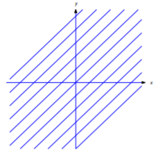
Example 4.5.2
For each value of the parameter c the equation
y=x+c
defines a line with slope 1(Figure 4.5.2).
Theorem 4.5.1
An equation that can be written in the form
H(x,y,c)=0
is said to define a one-parameter family of curves if, for each value of c in in some nonempty set of real numbers, the set of points (x,y) that satisfy Equation ??? forms a curve in the xy-plane.
Equations Equation ??? and Equation ??? define one–parameter families of curves. (Although Equation ??? isn’t in the form Equation ???, it can be written in this form as y−x−c=0.)
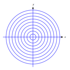
Example 4.5.3
If c>0, the graph of the equation
x2+y2−c=0
is a circle with center at (0,0) and radius √c. If c=0, the graph is the single point (0,0). (We don’t regard a single point as a curve.) If c<0, the equation has no graph. Hence, Equation ??? defines a one–parameter family of curves for positive values of c. This family consists of all circles centered at (0,0) (Figure 4.5.3).
Example 4.5.4
The equation
x2+y2+c2=0
does not define a one-parameter family of curves, since no (x,y) satisfies the equation if c≠0, and only the single point (0,0) satisfies it if c=0.
Recall from Section 1.2 that the graph of a solution of a differential equation is called an integral curve of the equation. Solving a first order differential equation usually produces a one–parameter family of integral curves of the equation. Here we are interested in the converse problem: given a one–parameter family of curves, is there a first order differential equation for which every member of the family is an integral curve. This suggests the next definition.
Theorem 4.5.1
4.5.2 If every curve in a one-parameter family defined by the equation
H(x,y,c)=0
is an integral curve of the first order differential equation
F(x,y,y′)=0,
then Equation ??? is said to be a differential equation for the family.
To find a differential equation for a one–parameter family we differentiate its defining equation Equation ??? implicitly with respect to x, to obtain
Hx(x,y,c)+Hy(x,y,c)y′=0.
If this equation doesn’t, then it is a differential equation for the family. If it does contain c, it may be possible to obtain a differential equation for the family by eliminating c between Equation ??? and Equation ???.
Example 4.5.5
Find a differential equation for the family of curves defined by
y=cx2.
Solution
Differentiating Equation ??? with respect to x yields
y′=2cx.
Therefore c=y′/2x, and substituting this into Equation ??? yields
y=xy′2
as a differential equation for the family of curves defined by Equation ???. The graph of any function of the form y=cx2 is an integral curve of this equation.
The next example shows that members of a given family of curves may be obtained by joining integral curves for more than one differential equation.
Example 4.5.6
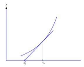
a. Try to find a differential equation for the family of lines tangent to the parabola y=x2.
b. Find two tangent lines to the parabola y=x2 that pass through (2,3), and find the points of tangency.
Solution
a. The equation of the line through a given point (x0,y0) with slope m is
y=y0+m(x−x0).
If (x0,y0) is on the parabola, then y0=x20 and the slope of the tangent line through (x0,x20) is m=2x0; hence, Equation ??? becomes
y=x20+2x0(x−x0),
or, equivalently,
y=−x20+2x0x.
Here x0 plays the role of the constant c in Definition 4.5.1; that is, varying x0 over (−∞,∞) produces the family of tangent lines to the parabola y=x2.
Differentiating Equation ??? with respect to x yields y′=2x0.. We can express x0 in terms of x and y by rewriting Equation ??? as
x20−2x0x+y=0
and using the quadratic formula to obtain
x0=x±√x2−y.
We must choose the plus sign in Equation ??? if x<x0 and the minus sign if x>x0; thus,
x0=(x+√x2−y)ifx<x0.
and
x0=(x−√x2−y)ifx>x0.
Since y′=2x0, this implies that
y′=2(x+√x2−y),ifx<x0
and
y′=2(x−√x2−y),ifx>x0.
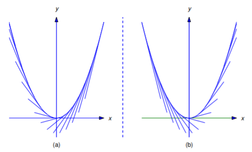
Neither Equation ??? nor Equation ??? is a differential equation for the family of tangent lines to the parabola y=x2. However, if each tangent line is regarded as consisting of two tangent half lines joined at the point of tangency, Equation ??? is a differential equation for the family of tangent half lines on which x is less than the abscissa of the point of tangency (Figure 4.5.4a), while Equation ??? is a differential equation for the family of tangent half lines on which x is greater than this abscissa (Figure 4.5.4(b)). The parabola y=x2 is also an integral curve of both Equation ??? and Equation ???.
b. From Equation ??? the point (x,y)=(2,3) is on the tangent line through (x0,x20) if and only if
3=−x20+4x0,
which is equivalent to
x20−4x0+3=(x0−3)(x0−1)=0.
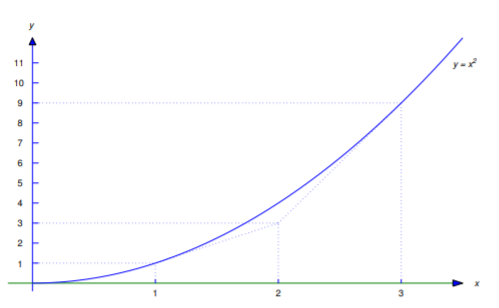
Letting x0=3 in Equation ??? shows that (2,3) is on the line
y=−9+6x,
which is tangent to the parabola at (x0,x20)=(3,9), as shown in Figure 4.5.5
Letting x0=1 in Equation ??? shows that (2,3) is on the line
y=−1+2x,
which is tangent to the parabola at (x0,x20)=(1,1), as shown in Figure 4.5.5.
Geometric Problems
We now consider some geometric problems that can be solved by means of differential equations.
Example 4.5.7
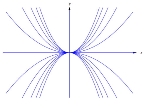
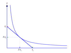
Find curves y=y(x) such that every point (x0,y(x0)) on the curve is the midpoint of the line segment with endpoints on the coordinate axes and tangent to the curve at (x0,y(x0)) (Figure 4.5.6).
Solution
The equation of the line tangent to the curve at P=(x0,y(x0) is
y=y(x0)+y′(x0)(x−x0).
If we denote the x and y intercepts of the tangent line by xI and yI (Figure 4.5.6), then
0=y(x0)+y′(x0)(xI−x0)
and
yI=y(x0)−y′(x0)x0.
From Figure 4.5.6, P is the midpoint of the line segment connecting (xI,0) and (0,yI) if and only if xI=2x0 and yI=2y(x0). Substituting the first of these conditions into Equation ??? or the second into Equation ??? yields
y(x0)+y′(x0)x0=0.
Since x0 is arbitrary we drop the subscript and conclude that y=y(x) satisfies
y+xy′=0,
which can be rewritten as
(xy)′=0.
Integrating yields xy=c, or
y=cx.
If c=0 this curve is the line y=0, which does not satisfy the geometric requirements imposed by the problem; thus, c≠0, and the solutions define a family of hyperbolas (Figure 4.5.7).
Example 4.5.8
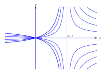
Find curves y=y(x) such that the tangent line to the curve at any point (x0,y(x0)) intersects the x-axis at (x20,0). Figure 4.5.8 illustrates the situation in the case where the curve is in the first quadrant and 0<x<1.
Solution
The equation of the line tangent to the curve at (x0,y(x0)) is
y=y(x0)+y′(x0)(x−x0).
Since (x20,0) is on the tangent line,
0=y(x0)+y′(x0)(x20−x0).
Since x0 is arbitrary we drop the subscript and conclude that y=y(x) satisfies
y+y′(x2−x)=0.
Therefore
y′y=−1x2−x=−1x(x−1)=1x−1x−1,
so
ln|y|=ln|x|−ln|x−1|+k=ln|xx−1|+k,
and
y=cxx−1.
If c=0, the graph of this function is the x-axis. If c≠0, it is a hyperbola with vertical asymptote x=1 and horizontal asymptote y=c. Figure 4.5.9 shows the graphs for c≠0.
Orthogonal Trajectories
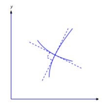
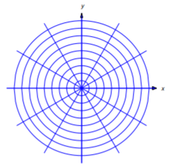
Two curves C1 and C2 are said to be orthogonal at a point of intersection (x0,y0) if they have perpendicular tangents at (x0,y0). (Figure 4.5.10). A curve is said to be an orthogonal trajectory of a given family of curves if it is orthogonal to every curve in the family. For example, every line through the origin is an orthogonal trajectory of the family of circles centered at the origin. Conversely, any such circle is an orthogonal trajectory of the family of lines through the origin (Figure 4.5.11).
Orthogonal trajectories occur in many physical applications. For example, if u=u(x,y) is the temperature at a point (x,y), the curves defined by
u(x,y)=c
are called isothermal curves. The orthogonal trajectories of this family are called heat-flow lines, because at any given point the direction of maximum heat flow is perpendicular to the isothermal through the point. If u represents the potential energy of an object moving under a force that depends upon (x,y), the curves Equation ??? are called equipotentials, and the orthogonal trajectories are called lines of force.
From analytic geometry we know that two nonvertical lines L1 and L2 with slopes m1 and m2, respectively, are perpendicular if and only if m2=−1/m1; therefore, the integral curves of the differential equation
y′=−1f(x,y)
are orthogonal trajectories of the integral curves of the differential equation
y′=f(x,y),
because at any point (x0,y0) where curves from the two families intersect the slopes of the respective tangent lines are
m1=f(x0,y0)andm2=−1f(x0,y0).
This suggests a method for finding orthogonal trajectories of a family of integral curves of a first order equation.
Finding Orthogonal Trajectories
- Step 1. Find a differential equation y′=f(x,y) for the given family.
- Step 2. Solve the differential equation y′=−1f(x,y) to find the orthogonal trajectories.
Example 4.5.9
Find the orthogonal trajectories of the family of circles
x2+y2=c2(c>0).
Solution
To find a differential equation for the family of circles we differentiate Equation ??? implicitly with respect to x to obtain
2x+2yy′=0,
or
y′=−xy.
Therefore the integral curves of
y′=yx
are orthogonal trajectories of the given family. We leave it to you to verify that the general solution of this equation is
y=kx,
where k is an arbitrary constant. This is the equation of a nonvertical line through (0,0). The y axis is also an orthogonal trajectory of the given family. Therefore every line through the origin is an orthogonal trajectory of the given family Equation ??? (Figure 4.5.11). This is consistent with the theorem of plane geometry which states that a diameter of a circle and a tangent line to the circle at the end of the diameter are perpendicular.
Example 4.5.10
Find the orthogonal trajectories of the family of hyperbolas
xy=c(c≠0)
(Figure 4.5.7).
Solution
Differentiating Equation ??? implicitly with respect to x yields
y+xy′=0,
or
y′=−yx;
thus, the integral curves of
y′=xy
are orthogonal trajectories of the given family. Separating variables yields
y′y=x
and integrating yields
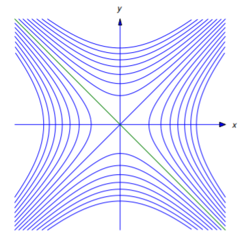
y2−x2=k,
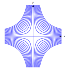
which is the equation of a hyperbola if k≠0, or of the lines y=x and y=−x if k=0 (Figure 4.5.12).
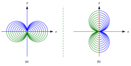
Example 4.5.11
Find the orthogonal trajectories of the family of circles defined by
(x−c)2+y2=c2(c≠0).
These circles are centered on the x-axis and tangent to the y-axis (Figure 4.5.13a).
Solution
Multiplying out the left side of Equation ??? yields
x2−2cx+y2=0,
and differentiating this implicitly with respect to x yields
2(x−c)+2yy′=0.
From Equation ???,
c=x2+y22x,
so
x−c=x−x2+y22x=x2−y22x.
Substituting this into Equation ??? and solving for y′ yields
y′=y2−x22xy.
The curves defined by Equation ??? are integral curves of Equation ???, and the integral curves of
y′=2xyx2−y2
are orthogonal trajectories of the family Equation ???. This is a homogeneous nonlinear equation, which we studied in Section 2.4. Substituting y=ux yields
u′x+u=2x(ux)x2−(ux)2=2u1−u2,
so
u′x=2u1−u2−u=u(u2+1)1−u2,
Separating variables yields
1−u2u(u2+1)u′=1x,
or, equivalently,
[1u−2uu2+1]u′=1x.
Therefore
ln|u|−ln(u2+1)=ln|x|+k.
By substituting u=y/x, we see that
ln|y|−ln|x|−ln(x2+y2)+ln(x2)=ln|x|+k,
which, since ln(x2)=2ln|x|, is equivalent to
ln|y|−ln(x2+y2)=k,
or
|y|=ek(x2+y2).
To see what these curves are we rewrite this equation as
x2+|y|2−e−k|y|=0
and complete the square to obtain
x2+(|y|−e−k/2)2=(e−k/2)2.
This can be rewritten as
x2+(y−h)2=h2,
where
h={e−k2 if y≥0,−e−k2 if y≤0.
Thus, the orthogonal trajectories are circles centered on the y axis and tangent to the x axis (Figure 4.5.13 (b)). The circles for which h>0 are above the x-axis, while those for which h<0 are below.