
3.4: Transformation of Functions


- Last updated
- Aug 8, 2022
- Save as PDF

( \newcommand{\kernel}{\mathrm{null}\,}\)
- Graph functions using vertical and horizontal shifts.
- Graph functions using reflections about the x-axis.
- Graph functions using compressions and stretches.
- Combine transformations.
We all know that a flat mirror enables us to see an accurate image of ourselves and whatever is behind us. When we tilt the mirror, the images we see may shift horizontally or vertically. But what happens when we bend a flexible mirror? Like a carnival funhouse mirror, it presents us with a distorted image of ourselves, stretched or compressed horizontally or vertically. In a similar way, we can distort or transform mathematical functions to better adapt them to describing objects or processes in the real world. In this section, we will take a look at several kinds of transformations.
Often when given a problem, we try to model the scenario using mathematics in the form of words, tables, graphs, and equations. One method we can employ is to adapt the basic graphs of the toolkit functions to build new models for a given scenario. There are systematic ways to alter functions to construct appropriate models for the problems we are trying to solve.
Identifying Vertical Shifts
One simple kind of transformation involves shifting the entire graph of a function up, down, right, or left. The simplest shift is a vertical shift, moving the graph up or down, because this transformation involves adding a positive or negative constant to the function. In other words, we add the same constant to the output value of the function regardless of the input. For a function g(x)=f(x)+k, the function f(x) is shifted vertically k units. See Figure 3.4.2 for an example.
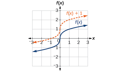
To help you visualize the concept of a vertical shift, consider that y=f(x). Therefore, f(x)+k is equivalent to y+k. Every unit of y is replaced by y+k, so the y-value increases or decreases depending on the value of k. The result is a shift upward or downward.
Given a function f(x), a new function g(x)=f(x)+k, where k is a constant, is a vertical shift of the function f(x). All the output values change by k units. If k is positive, the graph will shift up. If k is negative, the graph will shift down.
To regulate temperature in a green building, airflow vents near the roof open and close throughout the day. Figure 3.4.3 shows the area of open vents V (in square feet) throughout the day in hours after midnight, t. During the summer, the facilities manager decides to try to better regulate temperature by increasing the amount of open vents by 20 square feet throughout the day and night. Sketch a graph of this new function.
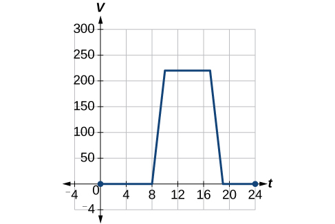
Solution
We can sketch a graph of this new function by adding 20 to each of the output values of the original function. This will have the effect of shifting the graph vertically up, as shown in Figure 3.4.4.
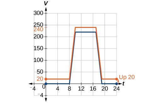
Notice that in Figure 3.4.4, for each input value, the output value has increased by 20, so if we call the new function S(t),we could write
S(t)=V(t)+20
This notation tells us that, for any value of t,S(t) can be found by evaluating the function V at the same input and then adding 20 to the result. This defines S as a transformation of the function V, in this case a vertical shift up 20 units. Notice that, with a vertical shift, the input values stay the same and only the output values change. See Table 3.4.1.
| t | 0 | 8 | 10 | 17 | 19 | 24 |
|---|---|---|---|---|---|---|
| V(t) | 0 | 0 | 220 | 220 | 0 | 0 |
| S(t) | 20 | 20 | 240 | 240 | 20 | 20 |
Given a tabular function, create a new row to represent a vertical shift.
- Identify the output row or column.
- Determine the magnitude of the shift.
- Add the shift to the value in each output cell. Add a positive value for up or a negative value for down.
A function f(x) is given in Table 3.4.2. Create a table for the function g(x)=f(x)−3.
| x | 2 | 4 | 6 | 8 |
|---|---|---|---|---|
| f(x) | 1 | 3 | 7 | 11 |
Solution
The formula g(x)=f(x)−3 tells us that we can find the output values of g by subtracting 3 from the output values of f. For example:
f(x)=1Giveng(x)=f(x)−3Given Transformationg(2)=f(2)−3=1−3=−2
Subtracting 3 from each f(x) value, we can complete a table of values for g(x) as shown in Table 3.4.3.
| x | 2 | 4 | 6 | 8 |
|---|---|---|---|---|
| f(x) | 1 | 3 | 7 | 11 |
| g(x) | -2 | 0 | 4 | 8 |
Analysis
As with the earlier vertical shift, notice the input values stay the same and only the output values change.
Exercise 3.4.1
The function h(t)=−4.9t2+30t gives the height h of a ball (in meters) thrown upward from the ground after t seconds. Suppose the ball was instead thrown from the top of a 10-m building. Relate this new height function b(t) to h(t), and then find a formula for b(t).
- Answer
-
b(t)=h(t)+10=−4.9t2+30t+10
Identifying Horizontal Shifts
We just saw that the vertical shift is a change to the output, or outside, of the function. We will now look at how changes to input, on the inside of the function, change its graph and meaning. A shift to the input results in a movement of the graph of the function left or right in what is known as a horizontal shift, shown in Figure 3.4.4.
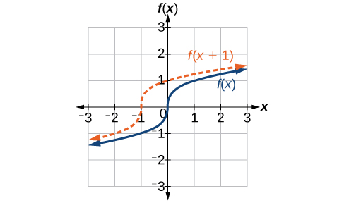
For example, if f(x)=x2, then g(x)=(x−2)2 is a new function. Each input is reduced by 2 prior to squaring the function. The result is that the graph is shifted 2 units to the right, because we would need to increase the prior input by 2 units to yield the same output value as given in f.
Given a function f, a new function g(x)=f(x−h), where h is a constant, is a horizontal shift of the function f. If h is positive, the graph will shift right. If h is negative, the graph will shift left.
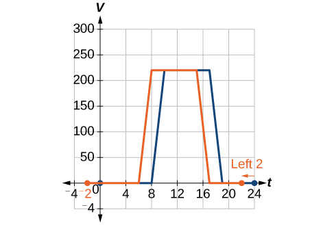
Returning to our building airflow example from Figure 3.4.2, suppose that in autumn the facilities manager decides that the original venting plan starts too late, and wants to begin the entire venting program 2 hours earlier. Sketch a graph of the new function.
Solution
We can set V(t) to be the original program and F(t) to be the revised program.
V(t)= the original venting plan
F(t)= starting 2 hrs sooner
In the new graph, at each time, the airflow is the same as the original function V was 2 hours later. For example, in the original function V, the airflow starts to change at 8 a.m., whereas for the function F, the airflow starts to change at 6 a.m. The comparable function values are V(8)=F(6). See Figure 3.4.5. Notice also that the vents first opened to 220ft2 at 10 a.m. under the original plan, while under the new plan the vents reach 220ft2 at 8 a.m., so V(10)=F(8).
In both cases, we see that, because F(t) starts 2 hours sooner, h=−2. That means that the same output values are reached when F(t)=V(t−(−2))=V(t+2).
Analysis
Note that V(t+2) has the effect of shifting the graph to the left.
Horizontal changes or “inside changes” affect the domain of a function (the input) instead of the range and often seem counterintuitive. The new function F(t) uses the same outputs as V(t), but matches those outputs to inputs 2 hours earlier than those of V(t). Said another way, we must add 2 hours to the input of V to find the corresponding output for F:F(t)=V(t+2).
Given a tabular function, create a new row to represent a horizontal shift.
- Identify the input row or column.
- Determine the magnitude of the shift.
- Add the shift to the value in each input cell.
A function f(x) is given in Table 3.4.4. Create a table for the function g(x)=f(x−3).
| x | 2 | 4 | 6 | 8 |
|---|---|---|---|---|
| f(x) | 1 | 3 | 7 | 11 |
Solution
The formula g(x)=f(x−3) tells us that the output values of g are the same as the output value of f when the input value is 3 less than the original value. For example, we know that f(2)=1. To get the same output from the function g, we will need an input value that is 3 larger. We input a value that is 3 larger for g(x) because the function takes 3 away before evaluating the function f.
g(5)=f(5−3)=f(2)=1
We continue with the other values to create Table 3.4.5.
| x | 5 | 7 | 9 | 11 |
|---|---|---|---|---|
| x−3 | 2 | 4 | 6 | 8 |
| f(x) | 1 | 3 | 7 | 11 |
| g(x) | 1 | 3 | 7 | 11 |
The result is that the function g(x) has been shifted to the right by 3. Notice the output values for g(x) remain the same as the output values for f(x), but the corresponding input values, x, have shifted to the right by 3. Specifically, 2 shifted to 5, 4 shifted to 7, 6 shifted to 9, and 8 shifted to 11.
Analysis
Figure 3.4.6 represents both of the functions. We can see the horizontal shift in each point.
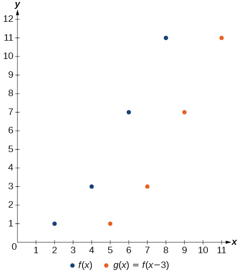
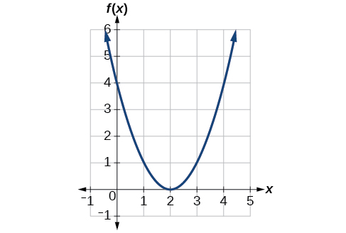
Figure 3.4.7 represents a transformation of the toolkit function f(x)=x2. Relate this new function g(x) to f(x), and then find a formula for g(x).
Solution
Notice that the graph is identical in shape to the f(x)=x2 function, but the x-values are shifted to the right 2 units. The vertex used to be at (0,0), but now the vertex is at (2,0). The graph is the basic quadratic function shifted 2 units to the right, so
g(x)=f(x−2)
Notice how we must input the value x=2 to get the output value y=0; the x-values must be 2 units larger because of the shift to the right by 2 units. We can then use the definition of the f(x) function to write a formula for g(x) by evaluating f(x−2).
f(x)=x2g(x)=f(x−2)g(x)=f(x−2)=(x−2)2
Analysis
To determine whether the shift is +2 or −2, consider a single reference point on the graph. For a quadratic, looking at the vertex point is convenient. In the original function, f(0)=0. In our shifted function, g(2)=0. To obtain the output value of 0 from the function f, we need to decide whether a plus or a minus sign will work to satisfy g(2)=f(x−2)=f(0)=0. For this to work, we will need to subtract 2 units from our input values.
The function G(m) gives the number of gallons of gas required to drive m miles. Interpret G(m)+10 and G(m+10)
Solution
G(m)+10 can be interpreted as adding 10 to the output, gallons. This is the gas required to drive m miles, plus another 10 gallons of gas. The graph would indicate a vertical shift.
G(m+10) can be interpreted as adding 10 to the input, miles. So this is the number of gallons of gas required to drive 10 miles more than m miles. The graph would indicate a horizontal shift.
Exercise 3.4.7
Given the function f(x)=√x, graph the original function f(x) and the transformation g(x)=f(x+2) on the same axes. Is this a horizontal or a vertical shift? Which way is the graph shifted and by how many units?
- Answer
-
The graphs of f(x) and g(x) are shown below. The transformation is a horizontal shift. The function is shifted to the left by 2 units.
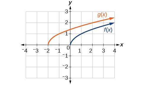
Figure 3.4.8
Combining Vertical and Horizontal Shifts
Now that we have two transformations, we can combine them together. Vertical shifts are outside changes that affect the output (y−) axis values and shift the function up or down. Horizontal shifts are inside changes that affect the input (x−) axis values and shift the function left or right. Combining the two types of shifts will cause the graph of a function to shift up or down and right or left.
Given a function and both a vertical and a horizontal shift, sketch the graph.
- Identify the vertical and horizontal shifts from the formula.
- The vertical shift results from a constant added to the output. Move the graph up for a positive constant and down for a negative constant.
- The horizontal shift results from a constant added to the input. Move the graph left for a positive constant and right for a negative constant.
- Apply the shifts to the graph in either order.
Given f(x)=|x|, sketch a graph of h(x)=f(x+1)−3.
Solution
The function f is our toolkit absolute value function. We know that this graph has a V shape, with the point at the origin. The graph of h has transformed f in two ways: f(x+1) is a change on the inside of the function, giving a horizontal shift left by 1, and the subtraction by 3 in f(x+1)−3 is a change to the outside of the function, giving a vertical shift down by 3. The transformation of the graph is illustrated in Figure 3.4.9.
Let us follow one point of the graph of f(x)=|x|.
- The point (0,0) is transformed first by shifting left 1 unit:(0,0)→(−1,0)
- The point (−1,0) is transformed next by shifting down 3 units:(−1,0)→(−1,−3)
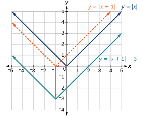
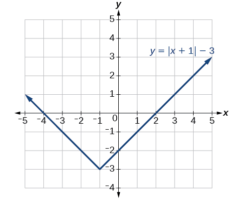
Figure 3.4.10 shows the graph of h.
Given f(x)=|x|, sketch a graph of h(x)=f(x−2)+4.
- Answer
-
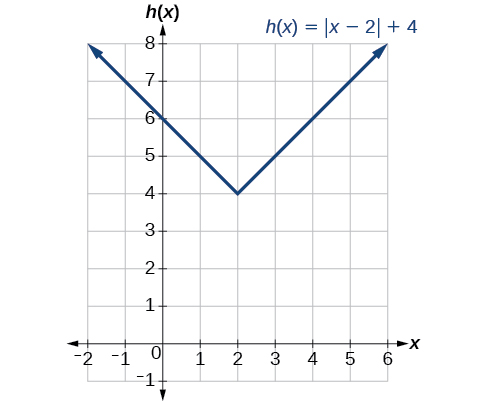
Figure 3.4.11
Write a formula for the graph shown in Figure 3.4.12, which is a transformation of the toolkit square root function.
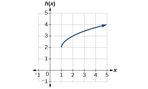
Solution
The graph of the toolkit function starts at the origin, so this graph has been shifted 1 to the right and up 2. In function notation, we could write that as
h(x)=f(x−1)+2
Using the formula for the square root function, we can write
h(x)=√x−1+2
Analysis
Note that this transformation has changed the domain and range of the function. This new graph has domain [1,∞) and range [2,∞).
Write a formula for a transformation of the toolkit reciprocal function f(x)=1x that shifts the function’s graph one unit to the right and one unit up.
- Answer
-
g(x)=1x−1+1
Graphing Functions Using Reflections about the Axes
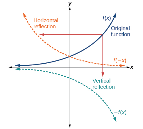
Another transformation that can be applied to a function is a reflection over the x- or y-axis. A vertical reflection reflects a graph vertically across the x-axis, while a horizontal reflection reflects a graph horizontally across the y-axis. The reflections are shown in Figure 3.4.13.
 .
.
Notice that the vertical reflection produces a new graph that is a mirror image of the base or original graph about the x-axis. The horizontal reflection produces a new graph that is a mirror image of the base or original graph about the y-axis.
Given a function f(x), a new function g(x)=−f(x) is a vertical reflection of the function f(x), sometimes called a reflection about (or over, or through) the x-axis.
Given a function, reflect the graph both vertically and horizontally.
- Multiply all outputs by –1 for a vertical reflection. The new graph is a reflection of the original graph about the x-axis.
Reflect the graph of s(t)=√t vertically.
Solution
a. Reflecting the graph vertically means that each output value will be reflected over the horizontal t-axis as shown in Figure 3.4.14.
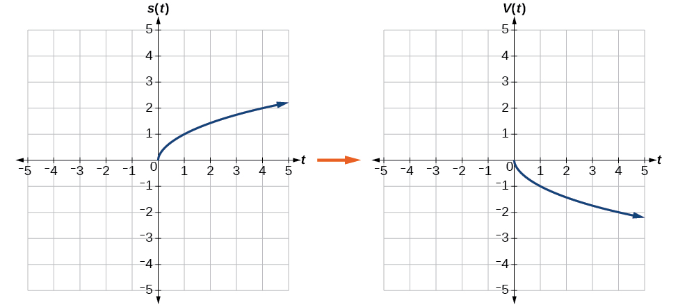
Because each output value is the opposite of the original output value, we can write
V(t)=−s(t) or V(t)=−√t
Notice that this is an outside change, or vertical shift, that affects the output s(t) values, so the negative sign belongs outside of the function.
Exercise 3.4.5
Reflect the graph of f(x)=|x−1| vertically
- Answer
-
a.
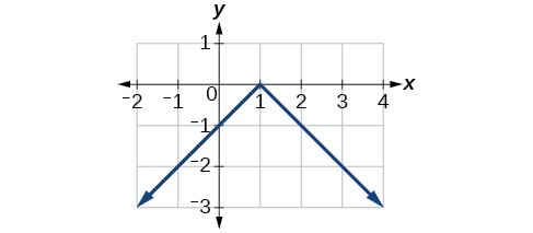
Figure 3.4.16: Graph of a vertically reflected absolute function. b.
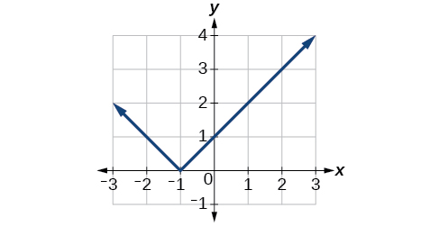
Figure 3.4.17: Graph of an absolute function translated one unit left.
A function f(x) is given as Table 3.4.6. Create a table for the functions below.
g(x)=−f(x)
| x | 2 | 4 | 6 | 8 |
|---|---|---|---|---|
| f(x) | 1 | 3 | 7 | 11 |
For g(x), the negative sign outside the function indicates a vertical reflection, so the x-values stay the same and each output value will be the opposite of the original output value. See Table 3.4.7.
| x | 2 | 4 | 6 | 8 |
|---|---|---|---|---|
| g(x) | -1 | -3 | -7 | -11 |
Exercise 3.4.6
A function f(x) is given as Table 3.4.9. Create a table for the functions below.
g(x)=−f(x)
| x | -2 | 0 | 2 | 4 |
|---|---|---|---|---|
| f(x) | 5 | 10 | 15 | 20 |
- Answer
-
a. g(x)=−f(x)
Table 3.4.10 x -2 0 2 4 g(x) -5 -10 -15 -20
Exercise 3.4.7
Given the toolkit function f(x)=x2, graph g(x)=−f(x). Take note of any surprising behavior for these functions.
- Answer
-
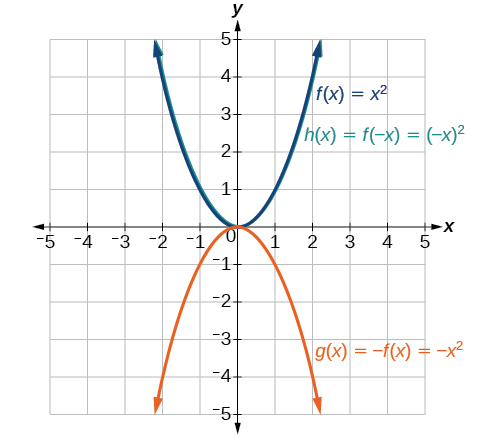
Figure 3.4.20: Graph of x2 and its reflections.
Graphing Functions Using Stretches and Compressions
Adding a constant to the inputs or outputs of a function changed the position of a graph with respect to the axes, but it did not affect the shape of a graph. We now explore the effects of multiplying the inputs or outputs by some quantity.
We can transform the inside (input values) of a function or we can transform the outside (output values) of a function. Each change has a specific effect that can be seen graphically.
Vertical Stretches and Compressions
When we multiply a function by a positive constant, we get a function whose graph is stretched or compressed vertically in relation to the graph of the original function. If the constant is greater than 1, we get a vertical stretch; if the constant is between 0 and 1, we get a vertical compression. Figure 3.4.23 shows a function multiplied by constant factors 2 and 0.5 and the resulting vertical stretch and compression.
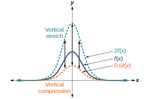
Given a function f(x), a new function g(x)=af(x), where a is a constant, is a vertical stretch or vertical compression of the function f(x).
- If a>1, then the graph will be stretched.
- If 0<a<1, then the graph will be compressed.
- If a<0, then there will be combination of a vertical stretch or compression with a vertical reflection.
Given a function, graph its vertical stretch.
- Identify the value of a.
- Multiply all range values by a
- If a>1, the graph is stretched by a factor of a.
- If 0<a<1, the graph is compressed by a factor of a.
- If a<0, the graph is either stretched or compressed and also reflected about the x-axis.
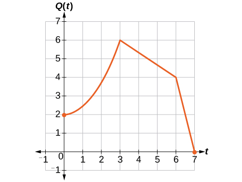
A function P(t) models the population of fruit flies. The graph is shown in Figure 3.4.24.
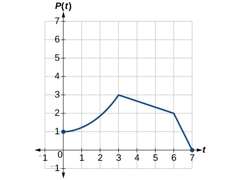
A scientist is comparing this population to another population, Q, whose growth follows the same pattern, but is twice as large. Sketch a graph of this population.
Solution
Because the population is always twice as large, the new population’s output values are always twice the original function’s output values. Graphically, this is shown in Figure 3.4.25.
If we choose four reference points, (0,1), (3,3), (6,2) and (7,0) we will multiply all of the outputs by 2.
The following shows where the new points for the new graph will be located.
(0,1)→(0,2)
(3,3)→(3,6)
(6,2)→(6,4)
(7,0)→(7,0)
Symbolically, the relationship is written as
Q(t)=2P(t)
This means that for any input t, the value of the function Q is twice the value of the function P. Notice that the effect on the graph is a vertical stretching of the graph, where every point doubles its distance from the horizontal axis. The input values, t, stay the same while the output values are twice as large as before.
Given a tabular function and assuming that the transformation is a vertical stretch or compression, create a table for a vertical compression.
- Determine the value of a.
- Multiply all of the output values by a.
A function f is given as Table 3.4.12. Create a table for the function g(x)=12f(x).
| x | 2 | 4 | 6 | 8 |
|---|---|---|---|---|
| f(x) | 1 | 3 | 7 | 11 |
Solution
The formula g(x)=12f(x) tells us that the output values of g are half of the output values of f with the same inputs. For example, we know that f(4)=3. Then
g(4)=12f(4)=12(3)=32
We do the same for the other values to produce Table 3.4.13.
| x | 2 | 4 | 6 | 8 |
|---|---|---|---|---|
| g(x) | 12 | 32 | 72 | 112 |
Analysis
The result is that the function g(x) has been compressed vertically by 12. Each output value is divided in half, so the graph is half the original height.
Exercise 3.4.9
A function f is given as Table 3.4.14. Create a table for the function g(x)=34f(x).
| x | 2 | 4 | 6 | 8 |
|---|---|---|---|---|
| f(x) | 12 | 16 | 20 | 0 |
- Answer
-
Table 3.4.15 x 2 4 6 8 g(x) 9 12 15 0
The graph in Figure 3.4.26 is a transformation of the toolkit function f(x)=x3. Relate this new function g(x) to f(x), and then find a formula for g(x).
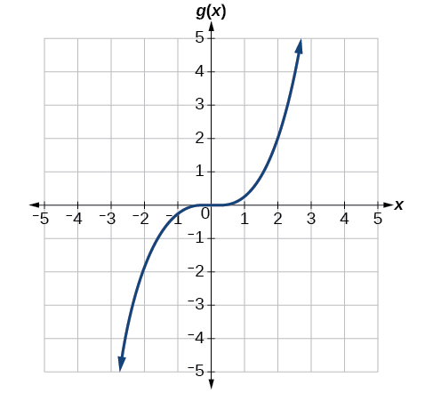
When trying to determine a vertical stretch or shift, it is helpful to look for a point on the graph that is relatively clear. In this graph, it appears that g(2)=2. With the basic cubic function at the same input, f(2)=23=8. Based on that, it appears that the outputs of g are 14 the outputs of the function f because g(2)=14f(2). From this we can fairly safely conclude that g(x)=14f(x).
We can write a formula for g by using the definition of the function f.
g(x)=14f(x)=14x3.
Exercise 3.4.1
Write the formula for the function that we get when we stretch the identity toolkit function by a factor of 3, and then shift it down by 2 units.
- Answer
-
g(x)=3x−2
Performing a Sequence of Transformations
When combining transformations, it is very important to consider the order of the transformations. For example, vertically shifting by 3 and then vertically stretching by 2 does not create the same graph as vertically stretching by 2 and then vertically shifting by 3, because when we shift first, both the original function and the shift get stretched, while only the original function gets stretched when we stretch first.
When we see an expression such as 2f(x)+3, which transformation should we start with? The answer here follows nicely from the order of operations. Given the output value of f(x), we first multiply by 2, causing the vertical stretch, and then add 3, causing the vertical shift. In other words, multiplication before addition.
- When combining vertical transformations written in the form af(x)+k, first vertically stretch by a and then vertically shift by k.
- Horizontal and vertical transformations are independent. It does not matter whether horizontal or vertical transformations are performed first.
Given Table 3.4.18 for the function f(x), create a table of values for the function g(x)=2f(3x)+1.
| x | 6 | 12 | 18 | 24 |
|---|---|---|---|---|
| f(x) | 10 | 14 | 15 | 17 |
Solution
There are three steps to this transformation, and we will work from the inside out. Starting with the horizontal transformations, f(3x) is a horizontal compression by 13, which means we multiply each x-value by 13.See Table 3.4.19.
| x | 2 | 4 | 6 | 8 |
|---|---|---|---|---|
| f(3x) | 10 | 14 | 15 | 17 |
Looking now to the vertical transformations, we start with the vertical stretch, which will multiply the output values by 2. We apply this to the previous transformation. See Table 3.4.20.
| x | 2 | 4 | 6 | 8 |
|---|---|---|---|---|
| 2f(3x) | 20 | 28 | 30 | 34 |
Finally, we can apply the vertical shift, which will add 1 to all the output values. See Table 3.4.21.
| x | 2 | 4 | 6 | 8 |
|---|---|---|---|---|
| g(x)=2f(3x)+1+1 | 21 | 29 | 31 | 35 |
Key Equations
- Vertical shift g(x)=f(x)+k (up for k>0)
- Horizontal shift g(x)=f(x−h)(right) for h>0
- Vertical reflection g(x)=−f(x)
- Horizontal reflection g(x)=f(−x)
- Vertical stretch g(x)=af(x) (a>0 )
- Vertical compression g(x)=af(x) (0<a<1)
Key Concepts
- A function can be shifted vertically by adding a constant to the output.
- A function can be shifted horizontally by adding a constant to the input.
- Relating the shift to the context of a problem makes it possible to compare and interpret vertical and horizontal shifts.
- Vertical and horizontal shifts are often combined.
- A vertical reflection reflects a graph about the x-axis. A graph can be reflected vertically by multiplying the output by –1.
- A function presented in tabular form can also be reflected by multiplying the values in the output rows or columns accordingly.
- A function presented as an equation can be reflected by applying transformations one at a time.
- A function can be compressed or stretched vertically by multiplying the output by a constant.
- The order in which different transformations are applied does affect the final function. Both vertical and horizontal transformations must be applied in the order given. However, a vertical transformation may be combined with a horizontal transformation in any order.
Glossary
horizontal compression
a transformation that compresses a function’s graph horizontally, by multiplying the input by a constant b>1
horizontal shift
a transformation that shifts a function’s graph left or right by adding a positive or negative constant to the input
vertical compression
a function transformation that compresses the function’s graph vertically by multiplying the output by a constant 0<a<1
vertical reflection
a transformation that reflects a function’s graph across the x-axis by multiplying the output by −1
vertical shift
a transformation that shifts a function’s graph up or down by adding a positive or negative constant to the output
vertical stretch
a transformation that stretches a function’s graph vertically by multiplying the output by a constant a>1