3.1: Graphs of Polynomials

Prerequisite Skillbuilders

The following topics are assumed knowledge prior to going through this material or the homework. If you find you are stuck on a concept, you might find the necessary remediation within these videos.

• What is a polynomial function?

Math 370 Learning Objectives

• Applications Involving Polynomial Functions: Develop models involving polynomial functions and use them to investigate and optimize values.
• End Behavior of Monomials: Review the end behavior of monomials.
• End Behavior of Polynomials: Review the end behavior of polynomials and how they are related to the end behavior of monomials.
• Middle Behavior of Polynomials: Review zeros of polynomials and how to find them.
• Sketching Graphs of Polynomials: Review basic techniques for sketching the graph of a polynomial function.

---

Introduction to Polynomial Functions

Three of the families of functions studied thus far – constant, linear, and quadratic – belong to a much larger group of functions called polynomials. We begin our formal study of general polynomials with a definition and some examples.

Definition: Polynomial Function

A polynomial function is a function of the form

\[f(x)=a_{n} x^{n}+a_{n-1} x^{n-1}+\ldots+a_{2} x^{2}+a_{1} x+a_{0},\label{PolyFunc} \]

where \(a_0\), \(a_{1}\), …, \(a_{n}\) are real numbers and \(n \geq 1\) is a natural number. The domain of a polynomial function is \((-\infty, \infty)\).

There are several things about the definition of a polynomial function that may be off-putting or downright frightening. The best thing to do is look at an example. Consider

\[f(x) = 4x^5 - 3x^2 + 2x - 5.\nonumber \]

Is this a polynomial function? We can re-write the formula for \(f\) as

\[f(x)= 4x^5 + 0 x^{4} + 0 x^{3} + (-3)x^2 + 2 x + (-5).\nonumber \]

Comparing this with Equation \( \ref{PolyFunc} \), we identify \(n=5\), \(a_{5} = 4\), \(a_{4} = 0\), \(a_{3} = 0\), \(a_{2} = -3\), \(a_{1} = 2\) and \(a_0 = -5\). In other words, \(a_{5}\) is the coefficient of \(x^{5}\), \(a_{4}\) is the coefficient of \(x^{4}\), and so forth; the subscript on the \(a\)’s merely indicates to which power of \(x\) the coefficient belongs. The business of restricting \(n\) to be a natural number lets us focus on well-behaved algebraic animals,

Example \( \PageIndex{1} \)

Determine if the following functions are polynomials. Explain your reasoning.

1. \(g(x) = \dfrac{4+x^3}{x}\)
2. \(p(x) = \dfrac{4x+x^3}{x}\)
3. \(q(x) = \dfrac{4x+x^3}{x^2+4}\)
4. \(f(x) =\sqrt[3]{x}\)
5. \(h(x) = |x|\)
6. \(z(x) = 0\)

Solution

1. We note directly that the domain of \(g(x) = \dfrac{x^3+4}{x}\) is \(x \neq 0\). By definition, a polynomial has all real numbers as its domain. Hence, \(g\) can’t be a polynomial.
2. Even though \(p(x) = \dfrac{x^3+4x}{x}\) simplifies to \(p(x) = x^2+4\), which certainly looks like the form given in Equation \( \ref{PolyFunc} \), the domain of \(p\), which, as you may recall, we determine before we simplify, excludes \(0\). Alas, \(p\) is not a polynomial function for the same reason \(g\) isn’t.
3. After what happened with \(p\) in the previous part, you may be a little shy about simplifying \(q(x) = \dfrac{x^3+4x}{x^2+4}\) to \(q(x) = x\), which certainly fits Equation \( \ref{PolyFunc} \). If we look at the domain of \(q\) before we simplified, we see that it is, indeed, all real numbers. A function which can be written in the form of Equation \( \ref{PolyFunc}  \) whose domain is all real numbers is, in fact, a polynomial. Therefore, this is a polynomial!
4. We can rewrite \(f(x) =\sqrt[3]{x}\) as \(f(x) = x^{\dfrac{1}{3}}\). Since \(\dfrac{1}{3}\) is not a natural number, \(f\) is not a polynomial.
5. The function \(h(x) = |x|\) isn’t a polynomial, since it can’t be written as a combination of powers of \(x\) even though it can be written as a piecewise function involving polynomials. As we shall see in this section, graphs of polynomials possess a quality that the graph of \(h\) does not.
6. There’s nothing in the definition of a polynomial function which prevents all the coefficients \(a_{n}\), etc., from being \(0\). Hence, \(z(x) = 0\), is an honest-to-goodness polynomial.

Definition: Degree, Leading Term, Leading Coefficient, and Constant Term of a Polynomial Function

Suppose \(f\) is a polynomial function.

• Given \(f(x)=a_{n} x^{n}+a_{n-1} x^{n-1}+\ldots+a_{2} x^{2}+a_{1} x+a_{0} \text { with } a_{n} \neq 0\), we say
  • The natural number \(n\) is called the degree of the polynomial \(f\).
  • The term \(a_{n} x^{n}\) is called the leading term of the polynomial \(f\).
  • The real number \(a_{n}\) is called the leading coefficient of the polynomial \(f\).
  • The real number \(a_0\) is called the constant term of the polynomial \(f\).
• If \(f(x) = a_0\), and \(a_0 \neq 0\), we say \(f\) has degree \(0\).
• If \(f(x) = 0\), we say \(f\) has no degree.

The reader may wonder why we have chosen to separate off constant functions from the other polynomials in our defintion above. Why not just lump them all together and, instead of forcing \(n\) to be a natural number, \(n = 1, 2, \ldots\), allow \(n\) to be a whole number, \(n = 0, 1, 2, \ldots\)? We could unify all of the cases, since, after all, isn’t \(a_0x^{0} = a_0\)?

The answer is "yes, as long as \(x\neq 0\)."

The functions \(f(x) = 3\) and \(g(x) = 3x^{0}\) are different, because their domains are different. The number \(f(0) = 3\) is defined, whereas \(g(0) = 3(0)^{0}\) is not.¹ Indeed, much of the theory we will develop in this chapter doesn’t include the constant functions, so we might as well treat them as outsiders from the start. One good thing that comes from our definition above is that we can now think of linear functions as degree \(1\) (or "first-degree") polynomial functions and quadratic functions as degree \(2\) (or "second-degree") polynomial functions.

Example \( \PageIndex{2} \)

Find the degree, leading term, leading coefficient and constant term of the following polynomial functions.

1. \(f(x) = 4x^5 - 3x^2 + 2x - 5\)
2. \(g(x) = 12x +x^3\)
3. \(h(x) = \dfrac{4-x}{5}\)
4. \(p(x) = (2x-1)^{3}(x-2)(3x+2)\)

Solution

1. There are no surprises with \(f(x) = 4x^5 - 3x^2 + 2x - 5\). It is written in the form of Equation \( \ref{PolyFunc} \), and we see that the degree is \(5\), the leading term is \(4x^5\), the leading coefficient is \(4\) and the constant term is \(-5\).
2. The form given in Equation \( \ref{PolyFunc} \) has the highest power of \(x\) first. To that end, we re-write \(g(x) = 12x +x^3 = x^3+12x\), and see that the degree of \(g\) is \(3\), the leading term is \(x^3\), the leading coefficient is \(1\) and the constant term is \(0\).
3. We need to rewrite the formula for \(h\) so that it resembles the form given in Equation \( \ref{PolyFunc} \): \[h(x) = \dfrac{4-x}{5} = \dfrac{4}{5} - \dfrac{x}{5} = -\dfrac{1}{5} x + \dfrac{4}{5}. \nonumber \]The degree of \(h\) is \(1\), the leading term is \(-\dfrac{1}{5} x\), the leading coefficient is \(-\dfrac{1}{5}\) and the constant term is \(\dfrac{4}{5}\).
4. It may seem that we have some work ahead of us to get \(p\) in the form of Equation \( \ref{PolyFunc} \). However, it is possible to glean the information requested about \(p\) without multiplying out the entire expression \((2x-1)^{3}(x-2)(3x+2)\). The leading term of \(p\) will be the term which has the highest power of \(x\). The way to get this term is to multiply the terms with the highest power of \(x\) from each factor together - in other words, the leading term of \(p(x)\) is the product of the leading terms of the factors of \(p(x)\). Hence, the leading term of \(p\) is \((2x)^3(x)(3x) = 24x^5\).^b This means that the degree of \(p\) is \(5\) and the leading coefficient is \(24\). As for the constant term, we can perform a similar trick. The constant term is obtained by multiplying the constant terms from each of the factors \((-1)^3(-2)(2) = 4\).²

Subsection Footnotes

¹ Technically, \( 0^0 \) is an indeterminate form, which is a special case of being undefined. The authors realize this is beyond pedantry, but we wouldn’t mention it if we didn’t feel it was necessary.

² Whatever you do, please please please do not think we are saying \( (2x - 1)^3 = (2x)^2 - (1)^3 \). This is absolutely not true! In fact, \[ (2x - 1)^3 =  (2x - 1)(2x - 1)(2x - 1) = (2x - 1)(4x^2 -4x +1) = 8x^3 -16x^2 + 6x - 1. \nonumber \]We hope you see the difference.

---

Applications Involving Polynomial Functions

Our next example shows how polynomials of higher-degree arise "naturally" in even the most basic geometric applications.³

Example \( \PageIndex{3} \)

A box with no top is to be fashioned from a \(10\) inch \(\times\) \(12\) inch piece of cardboard by cutting out congruent squares from each corner of the cardboard and then folding the resulting tabs. Let \(x\) denote the length of the side of the square which is removed from each corner (see Figure \( \PageIndex{1} \)).

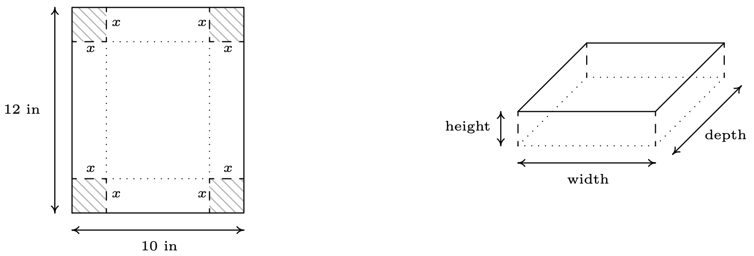
Figure \( \PageIndex{1} \)

1. Find the volume \(V\) of the box as a function of \(x\). Include an appropriate applied domain.
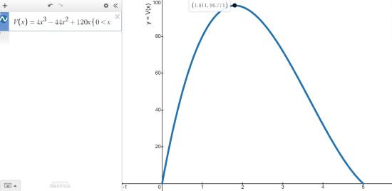
2. Use graphing technology to graph \(y=V(x)\) on the domain you found in part 1 and approximate the dimensions of the box with maximum volume to two decimal places. What is the maximum volume?

Solution

1. From Geometry, we know that \[\mbox{Volume} = \mbox{width} \times \mbox{height} \times \mbox{depth}.\nonumber\]The key is to find each of these quantities in terms of \(x\). From the Figure \( \PageIndex{1} \), we see that the height of the box is \(x\) itself. The cardboard piece is initially \(10\) inches wide. Removing squares with a side length of \(x\) inches from each corner leaves \(10-2x\) inches for the width.⁴ As for the depth, the cardboard is initially \(12\) inches long, so after cutting out \(x\) inches from each side, we would have \(12-2x\) inches remaining. As a function of \(x\),⁵ the volume is \[V(x) = x(10-2x)(12-2x) = 4x^3-44x^2+120x.\nonumber\]To find a suitable applied domain, we note that to make a box at all we need \(x > 0\). Also the shorter of the two dimensions of the cardboard is \(10\) inches, and since we are removing \(2x\) inches from this dimension, we also require \(10 - 2x > 0\) or \(x < 5\). Hence, our applied domain is \(0 < x < 5\).
2. Using Desmos, we see that the graph of \(y=V(x)\) has a relative maximum. For \(0 < x < 5\), this is also the absolute maximum. Clicking on the curve in Desmos, we find that this maximum occurs at approximately \( (1.811, 96.771)\). This yields a height of \(x \approx 1.81\) inches, a width of \(10 - 2x \approx 6.38\) inches, and a depth of \(12 - 2x \approx 8.38\) inches. The \(y\)-coordinate is the maximum volume, which is approximately \(96.77\) cubic inches (also written \(\mbox{in}^3\)).

Figure \( \PageIndex{2} \)

Subsection Footnotes

³ We understand that "naturally" is a very dangerous word in Mathematics.

⁴ There’s no harm in taking an extra step here and making sure this makes sense. If we chopped out a \(1\) inch square from each side, then the width would be \(8\) inches, so chopping out \(x\) inches would leave \(10−2x\) inches.

⁵ When we write \(V(x)\), it is in the context of function notation, not the volume \(V\) times the quantity \(x\).

---

End Behavior of Monomials

In order to solve Example \( \PageIndex{3} \), we made good use of the graph of the polynomial \(y=V(x)\), so we ought to turn our attention to graphs of polynomials in general. Figure \( \PageIndex{3} \) shows the graphs of \(y=x^2\), \(y=x^4\), and \(y=x^6\), side-by-side. We have omitted the axes to allow you to see that as the exponent increases, the "bottom" becomes "flatter" and the "sides" become "steeper." If you take the the time to graph these functions by hand, you will see why.⁶

Figure \( \PageIndex{3} \)

All of these functions are even,⁷ and it is exactly because the exponent is even.⁸ This symmetry is important, but we want to explore a different yet equally important feature of these functions which can be seen graphically – their end behavior.

The end behavior of a function is a way to describe what is happening to the function values (the \(y\)-values) as the \(x\)-values approach the "ends" of the \(x\)-axis.⁹ That is, what happens to \(y\) as \(x\) becomes negatively large without bound (written \(x \to -\infty\)) and, on the flip side, as \(x\) becomes positively large without bound (written \(x \to \infty\)).

For example, given \(f(x) = x^2\), as \(x \to -\infty\), we imagine substituting \(x=-100\), \(x=-1000\), etc., into \(f\) to get \(f(-100)=10000\), \(f(-1000)=1000000\), and so on. Thus the function values are becoming larger and larger positive numbers (without bound). To describe this behavior, we write: as \(x \to -\infty\), \(f(x) \to \infty\). If we study the behavior of \(f\) as \(x \to \infty\), we see that in this case, too, \(f(x) \to \infty\). (We told you that the symmetry was important!) The same can be said for any function of the form \(f(x) = x^n\) where \(n\) is an even natural number. If we generalize just a bit to include vertical scalings and reflections across the \(x\)-axis, we have the following theorem.

Theorem \(\PageIndex{1}\): End Behavior of \( f(x) = x^n \), where \( n \) is Even

Suppose \(f(x) = a x^{n}\) where \(a \neq 0\) is a real number and \(n\) is an even natural number. The end behavior of the graph of \(y=f(x)\) matches one of the following:

• for \(a > 0\), as \(x \to -\infty\), \(f(x) \to \infty\) and as \(x \to \infty\), \(f(x) \to \infty\)
• for \(a < 0\), as \(x \to -\infty\), \(f(x) \to -\infty\) and as \(x \to \infty\), \(f(x) \to -\infty\)

Graphically:

Figure \( \PageIndex{3} \)

We now turn our attention to functions of the form \(f(x) = x^{n}\) where \(n \geq 3\) is an odd natural number. (We ignore the case when \(n=1\), since the graph of \(f(x)=x\) is a line and doesn’t fit the general pattern of higher-degree odd polynomials.) The graphs of \(y=x^3\), \(y=x^5\), and \(y=x^7\) are shown in Figure \( \PageIndex{4} \). The "flattening" and "steepening" that we saw with the even powers presents itself here as well, and, it should come as no surprise that all of these functions are odd.¹⁰ The end behavior of these functions is all the same, with \(f(x) \to -\infty\) as \(x \to -\infty\) and \(f(x) \to \infty\) as \(x \to \infty\).

Figure \( \PageIndex{4} \)

As with the even degreed functions we studied earlier, we can generalize their end behavior.

Theorem \(\PageIndex{2}\): End Behavior of \( f(x) = x^n \), where \( n \) is Odd

Suppose \(f(x) = a x^{n}\) where \(a \neq 0\) is a real number and \(n \geq 3\) is an odd natural number. The end behavior of the graph of \(y=f(x)\) matches one of the following:

• for \(a > 0\), as \(x \to -\infty\), \(f(x) \to -\infty\) and as \(x \to \infty\), \(f(x) \to \infty\)
• for \(a < 0\), as \(x \to -\infty\), \(f(x) \to \infty\) and as \(x \to \infty\), \(f(x) \to -\infty\)

Graphically:

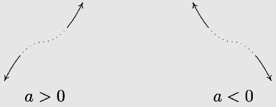
Figure \( \PageIndex{5} \)

Subsection Footnotes

⁶ Make sure you choose some \(x\)-values between \(−1\) and \(1\).

⁷ It's a good idea to review how to show a function is even or odd. This skill comes in very handy in calculus.

⁸ Herein lies one of the possible origins of the term "even" when applied to functions.

⁹ Of course, there are no ends to the \(x\)-axis.

¹⁰ And are, perhaps, the inspiration for the moniker "odd function."

---

The Intermediate Value Theorem

Despite having different end behavior, all functions of the form \(f(x) = ax^{n}\) for natural numbers \(n\) share two properties which help distinguish them from other animals in the algebra zoo: they are continuous and smooth. While these concepts are formally defined using Calculus,¹¹ informally, graphs of continuous functions have no "breaks" or "holes" in them, and the graphs of smooth functions have no "sharp turns." It turns out that these traits are preserved when functions are added together, so general polynomial functions inherit these qualities.

Figure \( \PageIndex{6}A \) shows the graph of a function which is neither smooth nor continuous, and Figure \( \PageIndex{6}B \) shows the graph of a polynomial, for comparison. The function in \( \PageIndex{6}A \) fails to be continuous where it has a "break" or "hole" in the graph; everywhere else, the function is continuous. The function is continuous at the "corner" and the "cusp," but we consider these "sharp turns," so these are places where the function fails to be smooth. Apart from these four places, the function is smooth and continuous. Polynomial functions are smooth and continuous everywhere, as exhibited in Figure \( \PageIndex{6}B \).

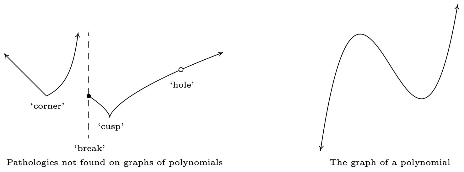
Figures \( \PageIndex{6}A \) (left) and \(  \PageIndex{6}B \) (right)

The notion of smoothness is what tells us graphically that, for example, \(f(x) = |x|\), whose graph is the characteristic "\(\vee\)" shape, cannot be a polynomial. The notion of continuity is what allowed us to construct the sign diagram for quadratic inequalities as we did in Section 2.4. This last result is formalized in the following theorem.

Theorem \(\PageIndex{2}\): Intermediate Value Theorem

Suppose \(f\) is a continuous function on an interval containing \(x=a\) and \(x=b\) with \(a<b\). If \(f(a)\) and \(f(b)\) have different signs, then \(f\) has at least one zero between \(x = a\) and \(x = b\); that is, for at least one real number \(c\) such that \(a < c < b\), we have \(f(c) = 0\).

The version of the Intermediate Value Theorem presented here is sometimes called the "Zero Version" due to the fact that it guarantees a continuous function that switches signs on the closed interval \( \left[ a, b \right] \) must have a zero on the open interval \( \left( a, b \right) \).

The Intermediate Value Theorem is extremely profound; it gets to the heart of what it means to be a real number, and is one of the most often used and underappreciated theorems in Mathematics. With that being said, most students see the result as common sense since it says, geometrically, that the graph of a polynomial function cannot be above the \(x\)-axis at one point and below the \(x\)-axis at another point without crossing the \(x\)-axis somewhere in between. The following example uses the Intermediate Value Theorem to establish a fact that that most students take for granted. Many students, and sadly some instructors, will find it silly.

Example \( \PageIndex{4} \)

Use the Intermediate Value Theorem to establish that \(\sqrt{2}\) is a real number.

Solution

Consider the polynomial function \[f(x) = x^2 - 2.\nonumber \]Then \(f(1) = -1\) and \(f(3) = 7\). Since \(f(1)\) and \(f(3)\) have different signs, the Intermediate Value Theorem guarantees us a real number \(c\) between \(1\) and \(3\) with \(f(c) = 0\). If \(c^2 - 2 = 0\) then \(c = \pm \sqrt{2}\). Since \(c\) is between \(1\) and \(3\), \(c\) is positive, so \(c = \sqrt{2}\) and, therefore, \( \sqrt{2} \) must be a real number.

Subsection Footnotes

¹¹ In fact, if you take Calculus, you’ll find that smooth functions are automatically continuous, so that saying "polynomials are continuous and smooth" is redundant.

---

End Behavior of Polynomials

Our primary use of the Intermediate Value Theorem is in the construction of sign diagrams, as in Section 2.4, since it guarantees us that polynomial functions are always positive \((+)\) or always negative \((-)\) on intervals which do not contain any of its zeros. The next example illustrates the procedure.

Example \( \PageIndex{5} \)

Construct a sign diagram for \(f(x) = x^3 (x-3)^2 (x+2) \left(x^2+1\right)\). Use it to give a rough sketch of the graph of \(y=f(x)\).

Solution

First, we find the zeros of \(f\) by solving \(x^3 (x-3)^2 (x+2)\left(x^2+1\right)=0\). We get \(x=0\), \(x=3\) and \(x=-2\). (The equation \(x^2+1=0\) produces no real solutions.) These three points divide the real number line into four intervals: \[(-\infty, -2), (-2,0), (0,3), \text{ and } (3,\infty).\nonumber \]We select the test values \(x=-3\), \(x=-1\), \(x=1\) and \(x=4\), and find that \(f(-3)\) is \((+)\), \(f(-1)\) is \((-)\) and \(f(1)\) is \((+)\) as is \(f(4)\). Wherever \(f\) is \((+)\), its graph is above the \(x\)-axis; wherever \(f\) is \((-)\), its graph is below the \(x\)-axis. The \(x\)-intercepts of the graph of \(f\) are \((-2,0)\), \((0,0)\) and \((3,0)\). Knowing \(f\) is smooth and continuous allows us to sketch its graph.

Figure \( \PageIndex{7} \)

A couple of notes about Example \( \PageIndex{5} \) are in order. First, note that we purposefully did not label the \(y\)-axis in the sketch of the graph of \(y=f(x)\). This is because the sign diagram gives us the zeros and the relative position of the graph - it doesn’t give us any information as to how high or low the graph strays from the \(x\)-axis. Furthermore, as we have mentioned earlier in the text, without Calculus, the values of the relative maximum and minimum can only be found approximately using a calculator. If we took the time to find the leading term of \(f\), we would find it to be \(x^8\). Looking at the end behavior of \(f\), we notice that it matches the end behavior of \(y=x^8\). This is no accident, as we find out in the next theorem.

Theorem \(\PageIndex{3}\): End Behavior of Polynomial Functions

The end behavior of a polynomial \(f(x)=a_{n} x^{n}+a_{n-1} x^{n-1}+\ldots+a_{2} x^{2}+a_{1} x+a_{0} \text { with } a_{n} \neq 0\) matches the end behavior of \(y = a_{n} x^{n}\).

To see why Theorem \( \PageIndex{3} \) is true, let’s first look at a specific example. Consider \(f(x) = 4x^3 - x + 5\). If we wish to examine end behavior, we look to see the behavior of \(f\) as \(x \to \pm \infty\). Since we’re concerned with \(x\)’s far down the \(x\)-axis, we are far away from \(x=0\) so can rewrite \(f(x)\) for these values of \(x\) as

\[f(x) = 4x^3 \left( 1 - \dfrac{1}{4x^2} + \dfrac{5}{4x^3}\right) \nonumber \]

As \(x\) becomes unbounded (in either direction), the terms \(\dfrac{1}{4x^2}\) and \(\dfrac{5}{4x^3}\) become closer and closer to \(0\), as the table below indicates.

\[\begin{array}{|r||r|r|} \hline x & \dfrac{1}{4x^2} & \dfrac{5}{4x^3} \vphantom{\dfrac{a}{a}} \\[4pt] \hline -1000 & 0.00000025 & -0.00000000125 \\ \hline -100 & 0.000025 & -0.00000125 \\ \hline -10 & 0.0025 & -0.00125 \\ \hline 10 & 0.0025 & 0.00125 \\ \hline 100 & 0.000025 & 0.00000125 \\ \hline 1000 & 0.00000025 & 0.00000000125 \\ \hline \end{array}\nonumber \]

In other words, as \(x \to \pm \infty\), \(f(x) \approx 4x^3\left( 1 - 0 +0\right) = 4x^3\), which is the leading term of \(f\). The formal proof of Theorem \( \PageIndex{3} \) works in much the same way. Factoring out the leading term leaves

\[f(x) = a_{n} x^{n} \left( 1 + \dfrac{a_{n - 1}}{a_{n} x}+ \ldots + \dfrac{a_2}{a_{n} x^{n-2}} + \dfrac{a_1}{a_{n} x^{n-1}}+\dfrac{a_0}{a_{n} x^{n}}\right)\nonumber \]

As \(x \to \pm \infty\), any term with an \(x\) in the denominator becomes closer and closer to \(0\), and we have \(f(x) \approx a_{n} x^{n}\). Geometrically, Theorem \( \PageIndex{3} \) says that if we graph \(y=f(x)\) using graphing technology, and continue to "zoom out," the graph of it and its leading term become indistinguishable. Figure \( \PageIndex{8} \) shows the graphs of \(y=4x^3-x+5\) (the solid blue line) and \(y=4x^3\) (the dashed black line) in two different windows.

  
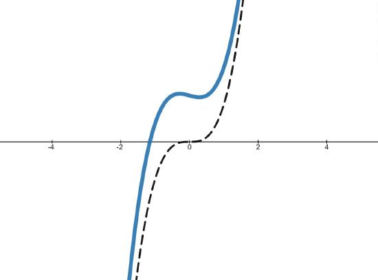
Figures \( \PageIndex{8}A \) (left) and \( \PageIndex{8}B \) (right)

---

Middle Behavior of Polynomials

Let’s return to the function in Example \( \PageIndex{5} \), \(f(x) = x^3 (x-3)^2 (x+2)\left(x^2+1\right)\), whose sign diagram and graph are reproduced in Figure \( \PageIndex{9} \) below for reference. Theorem \( \PageIndex{3} \) tells us that the end behavior is the same as that of its leading term, \(x^{8}\). This tells us that the graph of \(y=f(x)\) starts and ends above the \(x\)-axis. In other words, \(f(x)\) is \((+)\) as \(x \to \pm \infty\), and as a result, we no longer need to evaluate \(f\) at the test values \(x=-3\) and \(x=4\).

Is there a way to eliminate the need to evaluate \(f\) at the other test values? What we would really need to know is how the function behaves near its zeros - does it cross through the \(x\)-axis at these points, as it does at \(x=-2\) and \(x=0\), or does it simply touch and rebound like it does at \(x=3\). From the sign diagram, the graph of \(f\) will cross the \(x\)-axis whenever the signs on either side of the zero switch (like they do at \(x=-2\) and \(x=0\)); it will touch when the signs are the same on either side of the zero (as is the case with \(x=3\)). What we need to determine is the reason behind whether or not the sign change occurs.

Figure \( \PageIndex{9} \)

Fortunately, \(f\) was given to us in factored form: \(f(x) = x^3 (x-3)^2 (x+2)\). When we attempt to determine the sign of \(f(-4)\), we are attempting to find the sign of the number \((-4)^3 (-7)^2 (-2)\), which works out to be \((-)(+)(-)\) which is \((+)\). If we move to the other side of \(x=-2\), and find the sign of \(f(-1)\), we are determining the sign of \((-1)^3 (-4)^2 (+1)\), which is \((-)(+)(+)\) which gives us the \((-)\). Notice that signs of the first two factors in both expressions are the same in \(f(-4)\) and \(f(-1)\). The only factor which switches sign is the third factor, \((x+2)\), precisely the factor which gave us the zero \(x=-2\). If we move to the other side of \(0\) and look closely at \(f(1)\), we get the sign pattern \((+1)^3(-2)^2(+3)\) or \((+)(+)(+)\) and we note that, once again, going from \(f(-1)\) to \(f(1)\), the only factor which changed sign was the first factor, \(x^3\), which corresponds to the zero \(x=0\). Finally, to find \(f(4)\), we substitute to get \((+4)^3(+2)^2(+5)\) which is \((+)(+)(+)\) or \((+)\). The sign didn’t change for the middle factor \((x-3)^2\). Even though this is the factor which corresponds to the zero \(x=3\), the fact that the quantity is squared kept the sign of the middle factor the same on either side of \(3\).

If we look back at the exponents on the factors \((x+2)\) and \(x^3\), we see that they are both odd, so as we substitute values to the left and right of the corresponding zeros, the signs of the corresponding factors change which results in the sign of the function value changing. This is the key to the behavior of the function near the zeros. We need a definition and then a theorem.

Definition: Multiplicity

Suppose \(f\) is a polynomial function and \(m\) is a natural number. If \((x-c)^{m}\) is a factor of \(f(x)\) but \((x-c)^{m+1}\) is not, then we say \(x=c\) is a zero of multiplicity \(m\).

Hence, rewriting \[f(x) = x^3 (x-3)^2 (x+2)\nonumber \] as \[f(x) = (x-0)^3 (x-3)^2 (x-(-2))^{1},\nonumber \]we see that \(x=0\) is a zero of multiplicity \(3\), \(x=3\) is a zero of multiplicity \(2\) and \(x=-2\) is a zero of multiplicity \(1\).

Theorem \(\PageIndex{4}\): Basic Behavior of a Polynomial Graph Near a Zero of Multiplicity \( m \)

Suppose \(f\) is a polynomial function and \(x=c\) is a zero of multiplicity \(m\).

• If \(m\) is even, the graph of \(y=f(x)\) touches and rebounds from the \(x\)-axis at \((c,0)\).
• If \(m\) is odd, the graph of \(y=f(x)\) crosses through the \(x\)-axis at \((c,0)\).

Example \(\PageIndex{6}\)

Determine the zeros, their associated multiplicities, and the basic behavior for the function near the zeros if

\[ f(x) = 3x^2 (x - 2) (x + 4)^3 (x - 8)^{10}. \nonumber \]

Solution

Luckily, \( f \) has already been "prefactored" for us. Making a table of the zeros, their associated multiplicities, and the corresponding behavior of the graph at those zeros, we get

\[ \begin{array}{|c||c|c|}
\hline \text{Zero} & \text{Multiplicity} & \text{Basic Behavior} \\
\hline -4 & 3 & \text{crosses} \\
\hline 0 & 2 & \text{bounces} \\
\hline 2 & 1 & \text{crosses} \\
\hline 8 & 10 & \text{bounces} \\
\hline \end{array} \nonumber \]

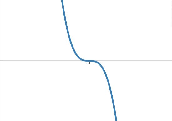
The graph of \( f(x) \) near each zero is shown in Figure \( \PageIndex{9} \).

  

  
Figures \( \PageIndex{9}A \) (upper left), \( \PageIndex{9}B \) (upper right), \( \PageIndex{9}C \) (lower left), and \( \PageIndex{9}D \) (lower right)
Zoomed in views of the zeros at \( x = -4 \), \( x = 0 \), \( x = 2 \), and \( x = 8 \), respectively.

Looking at Figure \( \PageIndex{9} \) in Example \( \PageIndex{6} \), we can see that there is more to "local behavior" near the zero of a function than just "crossing" or "bouncing." The following theorem completes our investigation into the graphs of polynomials.

Theorem \(\PageIndex{5}\): Exact Behavior of a Polynomial Graph Near a Zero of Multiplicity \( m \)

Suppose \(f\) is a polynomial function and \(x=c\) is a zero of multiplicity \(m\). The "local behavior" of the graph of \( f \) near \( x = c \) is that of either \( y = (x - c)^m \) or \( y = -(x - c)^m \).

 Determining if it is \( + \) or \( - \) in the equation \( y = \pm (x - c)^m \) comes from starting the graph of the function. An example is very useful here.

Example \(\PageIndex{7}\)

Determine the zeros, their associated multiplicities, and the exact behavior for the function near the zeros if

\[ f(x) = 3x^2 (x - 2) (x + 4)^3 (x - 8)^{10} \nonumber \]

Solution

We first note that the overall degree of this polynomial is \( 2 + 1 + 3 + 10 = 16 \), which is even. Moreover, the leading coefficient would be positive (in fact, it would be \( +3 \)). These two pieces of information alone tell us that \( f(x) \to \infty \) as \( x \to \pm \infty \).

The zeros for the polynomial are \( x = 0 \) (multiplicity \( 2 \)), \( x = 2 \) (multiplicity \( 1 \)), \( x = -4 \) (multiplicity \( 3 \)), and \( x = 8 \) (multiplicity \( 10 \)); however, listing these in numerical order will be helpful, so we begin our table.

\[ \begin{array}{|c||c|c|}
\hline \text{Zero} & \text{Multiplicity} & \text{Behavior} \\
\hline -4 & 3 &  \\
\hline 0 & 2 &  \\
\hline 2 & 1 &  \\
\hline 8 & 10 &  \\
\hline \end{array} \nonumber \]

We then use the multiplicities to fill in the "exact" behavior.

\[ \begin{array}{|c||c|c|}
\hline \text{Zero} & \text{Multiplicity} & \text{Behavior} \\
\hline -4 & 3 &  (x + 4)^3 \\
\hline 0 & 2 &  x^2 \\
\hline 2 & 1 &  x - 2 \\
\hline 8 & 10 & (x - 8)^{10} \\
\hline \end{array} \nonumber \]

Notice that I don't list whether the local behavior is like \( +(x - c)^m \) or \( -(x - c)^m \). This is because that behavior will show itself during the graphing process naturally. The following animation displays the graphing behavior from left-to-right.

---

Sketching Graphs of Polynomials

We have finally arrived at our goal - to accurately graph a polynomial function.¹² Our last example shows how end behavior and multiplicity allow us to sketch a decent graph without appealing to a sign diagram.

Example \( \PageIndex{8} \)

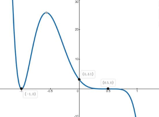
Sketch the graph of \(f(x) = -3.1(2x-1)^5(x+1)^2\) using end behavior and the multiplicity of its zeros.

Solution

The end behavior of the graph of \(f\) will match that of its leading term. To find the leading term, we multiply by the leading terms of each factor to get \((-3.1)(2x)(x)^2 = -6.2x^3\).¹³ This tells us that the graph will start above the \(x\)-axis, in Quadrant II, and finish below the \(x\)-axis, in Quadrant IV.

Next, we find the zeros of \(f\). Fortunately for us, \(f\) is factored.¹⁴ Listing the zeros, their multiplicities, and their local behaviors, we get the following table.

\[ \begin{array}{|c||c|c|}
\hline \text{Zero} & \text{Multiplicity} & \text{Behavior} \\
\hline -1 & 2 &  (x + 1)^2 \\
\hline \dfrac{1}{2} & 5 &  \left(x - \dfrac{1}{2}\right)^5 \\
\hline \end{array} \nonumber \]

Though we’re not asked to, we can find the \(y\)-intercept by finding \(f(0) = -3.1(2(0)-1)^5(0+1)^2 = 3.1\). Thus \((0,3.1)\) is an additional point on the graph.¹⁵ Putting this together gives us the graph in Figure \( \PageIndex{10} \).

Figure \( \PageIndex{10} \)

Subsection Footnotes

¹² In reality, we still need Calculus to determine where the maximums and minimums occur, but we have developed everything we can without the use of Calculus to get a fairly decent sketch.

¹³ In truth, there is no need to worry about the \( 3.1 \) or \( 2 \) in this product. The important part is the sign.

¹⁴ Obtaining the factored form of a polynomial is the main focus of the next few sections.

¹⁵ Finding the \( y \)-intercept in polynomial functions can either be simple (if the powers are low enough), or disastrously horrid (if the powers are large). You need to develop an intuitive sense of when finding the \( y \)-intercept is fruitful. Often, it's much better to just find the sign of the \( y \)-intercept so you can check that your polynomial graph is properly oriented.