9.2: Systems of Linear Equations - Augmented Matrices

An Introduction to Matrices

In Section 9.1 we introduced Gaussian Elimination as a means of transforming a system of linear equations into triangular form with the ultimate goal of producing an equivalent system of linear equations which is easier to solve. If we take a step back and study the process, we see that all of our moves are determined entirely by the coefficients of the variables involved, and not the variables themselves. Much the same thing happened when we studied long division in Section 3.2. Just as we developed synthetic division to streamline that process, in this section, we introduce a similar bookkeeping device to help us solve systems of linear equations. To that end, we define a matrix as a rectangular array of real numbers. We typically enclose matrices with square brackets, "\(\left[ \right.\)" and "\(\left. \right]\)," and we size matrices by the number of rows and columns they have. For example, the size (sometimes incorrectly called the dimension) of

\[\left[ \begin{array}{rrr}
3 & 0 & -1 \\
2 & -5 & 10 \\
\end{array} \right]\nonumber\]

is \(2 \times 3\) because it has \(2\) rows and \(3\) columns. The individual numbers in a matrix are called its entries and are usually labeled with double subscripts: the first tells which row the element is in and the second tells which column it is in. The rows are numbered from top to bottom and the columns are numbered from left to right. Matrices themselves are usually denoted by uppercase letters (\(\mathbf{A}\), \(\mathbf{B}\), \(\mathbf{C}\), etc.) while their entries are usually denoted by the corresponding letter. So, for instance, if we have

\[\mathbf{A} = \left[ \begin{array}{rrr}
3 & 0 & -1 \\
2 & -5 & 10 \\
\end{array} \right]\nonumber\]

then \(a_{11} = 3\), \(a_{12} = 0\), \(a_{13} = -1\), \(a_{21} = 2\), \(a_{22} = -5\), and \(a_{23} = 10\). While the theory of matrices takes up an entire course called Linear Algebra, we shall introduce them here solely as a bookkeeping device. Consider the system of linear equations from Example 9.1.2.b

\[\left\{ \begin{array}{lrcr}
(E1) & 2x+3y-z & = & 1 \\
(E2) & 10x-z & = & 2 \\
(E3) & 4x-9y+2z & = & 5 \\
\end{array} \right.\nonumber\]

We encode this system into a matrix by assigning each equation to a corresponding row. Within that row, each variable and the constant gets its own column, and to separate the variables on the left hand side of the equation from the constants on the right hand side, we use a vertical bar, \(\mid\). Note that in \(E2\), since \(y\) is not present, we record its coefficient as \(0\). The matrix associated with this system is

\[\begin{array}{c}
\begin{array}{rrrrrrr}
& & & \hspace{.33in} x & \hspace{.12in} y & \hspace{.1in} z & \hspace{.03in} c \\
\end{array} \\
\begin{array}{r}
(E1) \to \\ (E2) \to \\ (E3) \to \end{array} \left[ \begin{array}{rrr|r}
2 & 3 & -1 & 1\\
10 & 0 & -1 & 2 \\
4 & -9 & 2 & 5 \\
\end{array} \right]
\end{array}\nonumber\]

This matrix is called an augmented matrix because the column containing the constants is appended to the matrix containing the coefficients. In fact, the matrix containing the coefficients of the variables in the original linear system is called the coefficient matrix. The column of entries to the right side of the vertical bar is called the augmentation column.

To solve this system, we can use the same kind operations on the rows of the matrix that we performed on the equations of the system. More specifically, we have the following analog of Theorem 9.1.1 below.

Theorem \(\PageIndex{1}\): Row Operations

Given an augmented matrix for a system of linear equations, the following row operations produce an augmented matrix which corresponds to an equivalent system of linear equations.

• Interchange any two rows.
• Replace a row with a nonzero multiple of itself.¹
• Replace a row with itself plus a nonzero multiple of another row.²

As a demonstration of the moves in Theorem \( \PageIndex{1} \), we revisit some of the steps that were used in solving the systems of linear equations in Example 9.1.2 of Section 9.1. The reader is encouraged to perform the indicated operations on the rows of the augmented matrix to see that the machinations are identical to what is done to the coefficients of the variables in the equations. We first see a demonstration of switching two rows using the first step of Example 9.1.2.a.

\[\begin{array}{ccc}
\left\{ \begin{array}{lrcr}
(E1) & 3x-y+z & = & 3 \\
(E2) & 2x-4y+3z & = & 16 \\
(E3) & x-y+z & = & 5 \\
\end{array} \right. & \xrightarrow{\text{Switch $E1$ and $E3$}} & \left\{ \begin{array}{lrcr}
(E1) & x-y+z & = & 5 \\
(E2) & 2x-4y+3z & = & 16 \\
(E3) & 3x-y+z & = & 3 \\
\end{array} \right.
\end{array}\nonumber\]

\[\begin{array}{ccc}
\left[ \begin{array}{rrr|r}
3 & -1 & -1 & 3 \\
2 & -4 & 3 & 16 \\
1 & -1 & 1 & 5 \\
\end{array} \right] & \xrightarrow{\text{Switch $R1$ and $R3$}} & \left[ \begin{array}{rrr|r}
1 & -1 & -1 & 5 \\
2 & -4 & 3 & 16 \\
3 & -1 & 1 & 3 \\
\end{array} \right]
\end{array}\nonumber\]

Next, we have a demonstration of replacing a row with a nonzero multiple of itself using the first step of Example 9.1.2.c.

\[\begin{array}{ccc} \left\{ \begin{array}{lrcr} (E1) & 3x_1 +x_2 + x_4 & = & 6 \\ (E2) & 2x_1 + x_2 -x_3 & = & 4 \\ (E3) & x_2 -3x_3 -2x_4 & = & 0 \\ \end{array} \right. & \xrightarrow{\text{Replace $E1$ with $\frac{1}{3}E1$}} & \left\{ \begin{array}{lrcr} (E1) & x_1 + \frac{1}{3}x_2 + \frac{1}{3}x_4 & = & 2 \\ (E2) & 2x_1 + x_2 -x_3 & = & 4 \\ (E3) & x_2 -3x_3 -2x_4 & = & 0 \\ \end{array} \right. \end{array}\nonumber\]

\[\begin{array}{ccc} \left[ \begin{array}{rrrr|r} 3 & \hphantom{-} 1 & 0 & 1 & 6 \\ 2 & 1 & -1 & 0 & 4 \\ 0 & 1 & -3 & -2 & 0 \\ \end{array} \right] & \xrightarrow{\text{Replace $R1$ with $\frac{1}{3}R1$}} & \left[ \begin{array}{rrrr|r} 1 & \frac{1}{3} & 0 & \frac{1}{3} & 2 \\ 2 & \hphantom{-}1 & -1 & 0 & 4 \\ 0 & 1 & -3 & -2 & 0 \\ \end{array} \right] \end{array}\nonumber\]

Finally, we have an example of replacing a row with itself plus a multiple of another row using the second step from Example 9.1.2.b.

\[\begin{array}{ccc} \left\{ \begin{array}{lrcr} (E1) & x+\frac{3}{2}y-\frac{1}{2}z & = & \frac{1}{2} \\ (E2) & 10x-z & = & 2 \\ (E3) & 4x-9y+2z & = & 5 \\ \end{array} \right. & \xrightarrow[\text{Replace $E3$ with $-4E1 + E3$}]{\text{Replace $E2$ with $-10E1 + E2$}} & \left\{ \begin{array}{lrcr} (E1) & x+\frac{3}{2}y-\frac{1}{2}z & = & \frac{1}{2} \\ (E2) & -15y+4z & = & -3 \\ (E3) & -15y+4z & = & 3 \\ \end{array} \right. \end{array}\nonumber\]

\[\begin{array}{ccc} \left[ \begin{array}{rrr|r} 1 & \frac{3}{2} & -\frac{1}{2} & \frac{1}{2} \\ 10 & 0 & -1 & 2 \\ 4 & -9 & 2 & 5 \\ \end{array} \right] & \xrightarrow[\text{Replace $R3$ with $-4R1 + R3$}]{\text{Replace $R2$ with $-10R1 + R2$}} & \left[ \begin{array}{rrr|r} 1 & \frac{3}{2} & -\frac{1}{2} & \frac{1}{2} \\ 0 & -15 & 4 & -3 \\ 0 & -15 & 4 & 3 \\ \end{array} \right] \end{array}\nonumber\]

Subsection Footnotes

¹ That is, the row obtained by multiplying each entry in the row by the same nonzero number.

² Where we add entries in corresponding columns.

---

Row Echelon Form

The matrix equivalent of "triangular form" is row echelon form. The reader is encouraged to refer to the definition of triangular form for comparison. Note that the analog of "leading variable" of an equation is "leading entry" of a row. Specifically, the first nonzero entry (if it exists) in a row is called the leading entry of that row.

Definition: Row Echelon Form

A matrix is said to be in row echelon form provided all of the following conditions hold:

1. The leading entry of a given row must be to the right of the leading entry of the row above it.
2. Any row of all zeros cannot be placed above a row with nonzero entries.

Note

Some authors also require that all leading entries be \( 1 \) for a matrix to be in row echelon form. Strictly speaking, this is not necessary and, in fact, can lead to some atrocious calculations; however, if forcing a leading entry to be \( 1 \) doesn't cause too many fractional entries, then we will do that here.

To solve a system of a linear equations using an augmented matrix, we encode the system into an augmented matrix and apply Gaussian Elimination to the rows to get the matrix into row-echelon form. We then decode the matrix and back substitute. The next example illustrates this nicely.

Example \( \PageIndex{1} \)

Use an augmented matrix to transform the following system of linear equations into triangular form. Solve the system. \[\left\{ \begin{array}{rcl}
3x - y + z & = & 8 \\
x + 2y - z & = & 4 \\
2x+ 3y - 4z & = & 10 \\
\end{array} \right.\nonumber\]

Solution

We first encode the system into an augmented matrix.

\[\begin{array}{ccc} \left\{ \begin{array}{rcl} 3x - y + z & = & 8 \\ x + 2y - z & = & 4 \\ 2x+ 3y - 4z & = & 10 \\ \end{array} \right. & \xrightarrow{\text{Encode into the matrix}} & \left[ \begin{array}{rrr|r} 3 & -1 & 1 & 8 \\ 1 & 2 & -1 & 4 \\ 2 & 3 & -4 & 10 \\ \end{array} \right] \end{array}\nonumber\]

Thinking back to Gaussian Elimination at an equations level, our first order of business is to get \(x\) in \(E1\) with a coefficient of \(1\). At the matrix level, this means getting a leading \(1\) in \(R1\). To that end, we interchange \(R1\) and \(R2\).

\[\begin{array}{ccc} \left[ \begin{array}{rrr|r} 3 & -1 & 1 & 8 \\ 1 & 2 & -1 & 4 \\ 2 & 3 & -4 & 10 \\ \end{array} \right] & \xrightarrow{\text{Switch $R1$ and $R2$}} & \left[ \begin{array}{rrr|r} 1 & 2 & -1 & 4 \\ 3 & -1 & 1 & 8 \\ 2 & 3 & -4 & 10 \\ \end{array} \right] \end{array}\nonumber\]

Our next step is to eliminate the \(x\)’s from \(E2\) and \(E3\). From a matrix standpoint, this means we need \(0\)’s below the leading \(1\) in \(R1\). This guarantees the leading \(1\) in \(R2\) will be to the right of the leading \(1\) in \(R1\) in accordance with the first requirement of the definition of Row Echelon Form.

\[\begin{array}{ccc} \left[ \begin{array}{rrr|r} 1 & 2 & -1 & 4 \\ 3 & -1 & 1 & 8 \\ 2 & 3 & -4 & 10 \\ \end{array} \right] & \xrightarrow[\text{Replace $R3$ with $-2R1+R3$}]{\text{Replace $R2$ with $-3R1 +R2$}} & \left[ \begin{array}{rrr|r} 1 & 2 & -1 & 4 \\ 0 & -7 & 4 & -4 \\ 0 & -1 & -2 & 2 \\ \end{array} \right] \end{array}\nonumber\]

Now we repeat the above process for the variable \(y\) which means we need to get the leading entry in \(R2\) to be \(1\).

\[\begin{array}{ccc} \left[ \begin{array}{rrr|r} 1 & 2 & -1 & 4 \\ 0 & -7 & 4 & -4 \\ 0 & -1 & -2 & 2 \\ \end{array} \right] & \xrightarrow{\text{Replace $R2$ with $-\frac{1}{7}R2$}} & \left[ \begin{array}{rrr|r} 1 & 2 & -1 & 4 \\ 0 & 1 & -\frac{4}{7} & \frac{4}{7} \\ 0 & -1 & -2 & 2 \\ \end{array} \right] \end{array}\nonumber\]

To guarantee the leading \(1\) in \(R3\) is to the right of the leading \(1\) in \(R2\), we get a \(0\) in the second column of \(R3\).

\[\begin{array}{ccc} \left[ \begin{array}{rrr|r} 1 & 2 & -1 & 4 \\ 0 & 1 & -\frac{4}{7} & \frac{4}{7} \\ 0 & -1 & -2 & 2 \\ \end{array} \right] & \xrightarrow{\text{Replace $R3$ with $R2+R3$}} & \left[ \begin{array}{rrr|r} 1 & \hphantom{-}2 & -1 & 4 \\[4pt] 0 & 1 & -\frac{4}{7} & \frac{4}{7} \\[4pt] 0 & 0 & -\frac{18}{7} & \frac{18}{7} \\ \end{array} \right] \end{array}\nonumber\]

Finally, we get the leading entry in \(R3\) to be \(1\).

\[\begin{array}{ccc} \left[ \begin{array}{rrr|r} 1 & \hphantom{-}2 & -1 & 4 \\[4pt] 0 & 1 & -\frac{4}{7} & \frac{4}{7} \\[4pt] 0 & 0 & -\frac{18}{7} & \frac{18}{7} \\ \end{array} \right] & \xrightarrow{\text{Replace $R3$ with $-\frac{7}{18}R3$}} & \left[ \begin{array}{rrr|r} 1 & \hphantom{-}2 & -1 & 4 \\ 0 & 1 & -\frac{4}{7} & \frac{4}{7} \\ 0 & 0 &1 & -1 \\ \end{array} \right] \end{array}\nonumber\]

Decoding from the matrix gives a system in triangular form

\[\begin{array}{ccc} \left[ \begin{array}{rrr|r} 1 & \hphantom{-}2 & -1 & 4 \\ 0 & 1 & -\frac{4}{7} & \frac{4}{7} \\ 0 & 0 &1 & -1 \\ \end{array} \right] & \xrightarrow{\text{Decode from the matrix}} & \left \{ \begin{array}{rcr} x + 2y-z & = & 4 \\ y - \frac{4}{7} z & = & \frac{4}{7} \\ z & = & -1 \end{array} \right. \end{array}\nonumber\]

We get \(z=-1\), \(y = \frac{4}{7} z + \frac{4}{7} = \frac{4}{7}(-1)+\frac{4}{7} = 0\) and \(x = -2y+z+4 = -2(0)+(-1)+4 = 3\) for a final answer of \((3,0,-1)\). We leave it to the reader to check.

---

Reduced Row Echelon Form

As part of Gaussian Elimination, we used row operations to obtain \(0\)’s beneath each leading entry to put the matrix into row echelon form. If we also require that \(0\)’s are the only numbers above a leading entry, and if we require that all leading entries are \( 1 \), we have what is known as the reduced row echelon form of the matrix.

Definition: Reduced Row Echelon Form

A matrix is said to be in reduced row echelon form provided both of the following conditions hold:

1. The matrix is in row echelon form.
2. All leading entries are \( 1 \)s.
3. The leading \(1\)s are the only nonzero entry in their respective columns.

Of what significance is the reduced row echelon form of a matrix? To illustrate, let’s take the row echelon form from Example \( \PageIndex{1} \) and perform the necessary steps to put into reduced row echelon form. We start by using the leading \(1\) in \(R3\) to zero out the numbers in the rows above it.

\[\begin{array}{ccc} \left[ \begin{array}{rrr|r} 1 & \hphantom{-}2 & -1 & 4 \\ 0 & 1 & -\frac{4}{7} & \frac{4}{7} \\ 0 & 0 &1 & -1 \\ \end{array} \right] & \xrightarrow[\text{Replace $R2$ with $\frac{4}{7} R3 + R2$}]{\text{Replace $R1$ with $R3+R1$}} & \left[ \begin{array}{rrr|r} 1 & 2 & 0 & 3 \\ 0 & 1 & 0 & 0 \\ 0 & 0 &1 & -1 \\ \end{array} \right] \end{array}\nonumber\]

Finally, we take care of the \(2\) in \(R1\) above the leading \(1\) in \(R2\).

\[\begin{array}{ccc} \left[ \begin{array}{rrr|r} 1 & 2 & 0 & 3 \\ 0 & 1 & 0 & 0 \\ 0 & 0 &1 & -1 \\ \end{array} \right] & \xrightarrow{\text{Replace $R1$ with $-2R2+R1$}} & \left[ \begin{array}{rrr|r} 1 & 0 & 0 & 3 \\ 0 & 1 & 0 & 0 \\ 0 & 0 &1 & -1 \\ \end{array} \right] \end{array}\nonumber\]

To our surprise and delight, when we decode this matrix, we obtain the solution instantly without having to deal with any back-substitution at all.

\[\begin{array}{ccc} \left[ \begin{array}{rrr|r} 1 & 0 & 0 & 3 \\ 0 & 1 & 0 & 0 \\ 0 & 0 &1 & -1 \\ \end{array} \right] & \xrightarrow{\text{Decode from the matrix}} & \left\{ \begin{array}{rcr} x & = & 3 \\ y & = & 0 \\ z & = & -1 \end{array} \right. \end{array}\nonumber\]

Note that in the previous discussion, we could have started with \(R2\) and used it to get a zero above its leading \(1\) and then done the same for the leading \(1\) in \(R3\). By starting with \(R3\), however, we get more zeros first, and the more zeros there are, the faster the remaining calculations will be. It is also worth noting that while a matrix has several³ row echelon forms, it has only one reduced row echelon form. The process by which we have put a matrix into reduced row echelon form is called Gauss-Jordan Elimination.

Example \( \PageIndex{2} \)

Solve the following system using an augmented matrix. Use Gauss-Jordan Elimination to put the augmented matrix into reduced row echelon form.

\[\left \{ \begin{array}{rcr} x_2 - 3x_1 + x_4 & = & 2 \\ 2x_1 + 4x_3 & = & 5 \\ 4x_2-x_4 & = & 3 \end{array} \right.\nonumber\]

Solution

We first encode the system into a matrix. (Pay attention to the subscripts!)

\[\begin{array}{ccc} \left\{ \begin{array}{rcr} x_2 - 3x_1 + x_4 & = & 2 \\ 2x_1 + 4x_3 & = & 5 \\ 4x_2-x_4 & = & 3 \end{array} \right. & \xrightarrow{\text{Encode into the matrix}} & \left[ \begin{array}{rrrr|r} -3 & \hphantom{-}1 & \hphantom{-}0 & 1 & 2 \\ 2 & 0 & 4 & 0 & 5 \\ 0 & 4 & 0 & -1 & 3 \\ \end{array} \right] \end{array}\nonumber\]

Next, we get a leading \(1\) in the first column of \(R1\).

\[\begin{array}{ccc} \left[ \begin{array}{rrrr|r} -3 & \hphantom{-}1 & \hphantom{-}0 & 1 & 2 \\ 2 & 0 & 4 & 0 & 5 \\ 0 & 4 & 0 & -1 & 3 \\ \end{array} \right] & \xrightarrow{\text{Replace $R1$ with $-\frac{1}{3}R1$}} & \left[ \begin{array}{rrrr|r} 1 & -\frac{1}{3} & \hphantom{-}0 & -\frac{1}{3} & -\frac{2}{3} \\ 2 & 0 & 4 & 0 & 5 \\ 0 & 4 & 0 & -1 & 3 \\ \end{array} \right] \end{array}\nonumber\]

Now we eliminate the nonzero entry below our leading \(1\).

\[\begin{array}{ccc} \left[ \begin{array}{rrrr|r} 1 & -\frac{1}{3} & \hphantom{-}0 & -\frac{1}{3} & -\frac{2}{3} \\ 2 & 0 & 4 & 0 & 5 \\ 0 & 4 & 0 & -1 & 3 \\ \end{array} \right] & \xrightarrow{\text{Replace $R2$ with $-2R1+R2$}} & \left[ \begin{array}{rrrr|r} 1 & -\frac{1}{3} & \hphantom{-}0 & -\frac{1}{3} & -\frac{2}{3} \\[4pt] 0 & \frac{2}{3} & 4 & \frac{2}{3} & \frac{19}{3} \\[4pt] 0 & 4 & 0 & -1 & 3 \\ \end{array} \right] \end{array}\nonumber\]

We proceed to get a leading \(1\) in \(R2\).

\[\begin{array}{ccc} \left[ \begin{array}{rrrr|r} 1 & -\frac{1}{3} & \hphantom{-}0 & -\frac{1}{3} & -\frac{2}{3} \\[4pt] 0 & \frac{2}{3} & 4 & \frac{2}{3} & \frac{19}{3} \\[4pt] 0 & 4 & 0 & -1 & 3 \\ \end{array} \right] & \xrightarrow{\text{Replace $R2$ with $\frac{3}{2}R2$}} & \left[ \begin{array}{rrrr|r} 1 & -\frac{1}{3} & \hphantom{-}0 & -\frac{1}{3} & -\frac{2}{3} \\[4pt] 0 & 1 & 6 & 1 & \frac{19}{2} \\[4pt] 0 & 4 & 0 & -1 & 3 \\ \end{array} \right] \end{array}\nonumber\]

We now zero out the entry below the leading \(1\) in \(R2\).

\[\begin{array}{ccc} \left[ \begin{array}{rrrr|r} 1 & -\frac{1}{3} & \hphantom{-}0 & -\frac{1}{3} & -\frac{2}{3} \\[4pt] 0 & 1 & 6 & 1 & \frac{19}{2} \\[4pt] 0 & 4 & 0 & -1 & 3 \\ \end{array} \right] & \xrightarrow{\text{Replace $R3$ with $-4R2+R3$}} & \left[ \begin{array}{rrrr|r} 1 & -\frac{1}{3} & 0 & -\frac{1}{3} & -\frac{2}{3} \\[4pt] 0 & 1 & 6 & 1 & \frac{19}{2} \\[4pt] 0 & 0& -24 & -5 & -35 \\ \end{array} \right] \end{array}\nonumber\]

Next, it’s time for a leading \(1\) in \(R3\). \[\begin{array}{ccc} \left[ \begin{array}{rrrr|r} 1 & -\frac{1}{3} & 0 & -\frac{1}{3} & -\frac{2}{3} \\[4pt] 0 & 1 & 6 & 1 & \frac{19}{2} \\[4pt] 0 & 0& -24 & -5 & -35 \\ \end{array} \right] & \xrightarrow{\text{Replace $R3$ with $-\frac{1}{24}R3$}} & \left[ \begin{array}{rrrr|r} 1 & -\frac{1}{3} & \hphantom{-}0 & -\frac{1}{3} & -\frac{2}{3} \\[4pt] 0 & 1 & 6 & 1 & \frac{19}{2} \\[4pt] 0 & 0& 1 & \frac{5}{24} & \frac{35}{24} \\ \end{array} \right] \end{array}\nonumber\]

The matrix is now in row echelon form. To get the reduced row echelon form, we start with the last leading \(1\) we produced and work to get \(0\)’s above it. \[\begin{array}{ccc} \left[ \begin{array}{rrrr|r} 1 & -\frac{1}{3} & \hphantom{-}0 & -\frac{1}{3} & -\frac{2}{3} \\[4pt] 0 & 1 & 6 & 1 & \frac{19}{2} \\[4pt] 0 & 0& 1 & \frac{5}{24} & \frac{35}{24} \\ \end{array} \right]& \xrightarrow{\text{Replace $R2$ with $-6R3+R2$}} & \left[ \begin{array}{rrrr|r} 1 & -\frac{1}{3} & \hphantom{-}0 & -\frac{1}{3} & -\frac{2}{3} \\[4pt] 0 & 1 & 0 & -\frac{1}{4} & \frac{3}{4} \\[4pt] 0 & 0& 1 & \frac{5}{24} & \frac{35}{24} \\ \end{array} \right] \end{array}\nonumber\]

Lastly, we get a \(0\) above the leading \(1\) of \(R2\).

\[\begin{array}{ccc} \left[ \begin{array}{rrrr|r} 1 & -\frac{1}{3} & \hphantom{-}0 & -\frac{1}{3} & -\frac{2}{3} \\[4pt] 0 & 1 & 0 & -\frac{1}{4} & \frac{3}{4} \\[4pt] 0 & 0& 1 & \frac{5}{24} & \frac{35}{24} \\ \end{array} \right] & \xrightarrow{\text{Replace $R1$ with $\frac{1}{3}R2+R1$}} & \left[ \begin{array}{rrrr|r} 1 & \hphantom{-}0 & \hphantom{-}0 & -\frac{5}{12} & -\frac{5}{12} \\[4pt] 0 & 1 & 0 & -\frac{1}{4} & \frac{3}{4} \\[4pt] 0 & 0& 1 & \frac{5}{24} & \frac{35}{24} \\ \end{array} \right] \end{array}\nonumber\]

At last, we decode to get

\[\begin{array}{ccc} \left[ \begin{array}{rrrr|r} 1 & \hphantom{-}0 & \hphantom{-}0 & -\frac{5}{12} & -\frac{5}{12} \\[4pt] 0 & 1 & 0 & -\frac{1}{4} & \frac{3}{4} \\[4pt] 0 & 0& 1 & \frac{5}{24} & \frac{35}{24} \\ \end{array} \right] & \xrightarrow{\text{Decode from the matrix}} & \left\{ \begin{array}{rcr} x_1 - \frac{5}{12} x_4 & = & -\frac{5}{12} \\[4pt] x_2 - \frac{1}{4}x_4 & = & \frac{3}{4} \\[4pt] x_3 + \frac{5}{24} x_4 & = & \frac{35}{24} \end{array} \right. \end{array}\nonumber\]

We have that \(x_{4}\) is free and we assign it the parameter \(t\). We obtain \(x_{3} = -\frac{5}{24} t + \frac{35}{24}\), \(x_{2} = \frac{1}{4} t + \frac{3}{4}\), and \(x_{1} = \frac{5}{12}t - \frac{5}{12}\). Our solution is \(\left\{ \left( \frac{5}{12}t - \frac{5}{12}, \frac{1}{4} t + \frac{3}{4}, -\frac{5}{24} t + \frac{35}{24}, t \right) : -\infty < t < \infty \right\}\) and leave it to the reader to check.

Like all good algorithms, putting a matrix in row echelon or reduced row echelon form can easily be performed by technology. We use this in our next example.

Example \( \PageIndex{3} \)

Find the quadratic function passing through the points \((-1,3)\), \((2,4)\), \((5,-2)\).

Solution

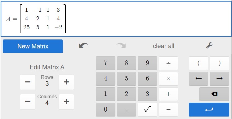
A quadratic function has the form \(f(x) =ax^2+bx+c\) where \(a \neq 0\). Our goal is to find \(a\), \(b\) and \(c\) so that the three given points are on the graph of \(f\). If \((-1,3)\) is on the graph of \(f\), then \(f(-1) = 3\), or \(a(-1)^2+b(-1) + c = 3\) which reduces to \(a-b+c=3\), an honest-to-goodness linear equation with the variables \(a\), \(b\) and \(c\). Since the point \((2,4)\) is also on the graph of \(f\), then \(f(2) = 4\) which gives us the equation \(4a+2b+c = 4\). Lastly, the point \((5,-2)\) is on the graph of \(f\) gives us \(25a+5b+c = -2\). Putting these together, we obtain a system of three linear equations. Encoding this into an augmented matrix produces \[\begin{array}{ccc} \left\{ \begin{array}{rcr} a-b+c & = & 3 \\ 4a+2b+c & = & 4 \\ 25a+5b+c & = & -2 \end{array} \right. & \xrightarrow{\text{Encode into the matrix}} & \left[ \begin{array}{rrr|r} 1 & -1 & \hphantom{-}1 & 3 \\ 4 & 2 & 1 & 4 \\ 25 & 5 & 1 & -2 \\ \end{array} \right] \end{array}\nonumber\]

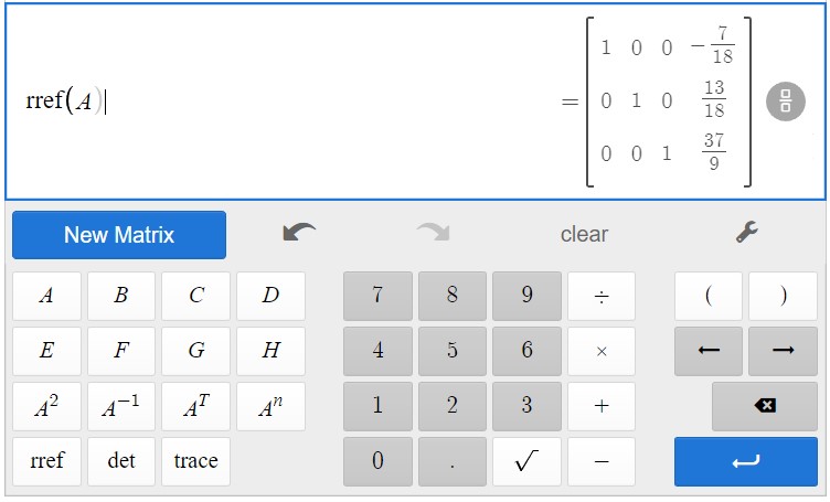
Using Desmos, we find \(a = -\frac{7}{18}\), \(b = \frac{13}{18}\) and \(c = \frac{37}{9}\). Hence, the one and only quadratic which fits the bill is \(f(x) = -\frac{7}{18} x^2 + \frac{13}{18} x + \frac{37}{9}\). To verify this analytically, we see that \(f(-1) = 3\), \(f(2) = 4\), and \(f(5) = -2\). We can use the calculator to check our solution as well by plotting the three data points and the function \(f\).

  

  

Subsection Footnotes

³ Infinite, in fact.