6.4: Logarithmic Equations and Inequalities
- Page ID
- 149181

\( \newcommand{\vecs}[1]{\overset { \scriptstyle \rightharpoonup} {\mathbf{#1}} } \)
\( \newcommand{\vecd}[1]{\overset{-\!-\!\rightharpoonup}{\vphantom{a}\smash {#1}}} \)
\( \newcommand{\id}{\mathrm{id}}\) \( \newcommand{\Span}{\mathrm{span}}\)
( \newcommand{\kernel}{\mathrm{null}\,}\) \( \newcommand{\range}{\mathrm{range}\,}\)
\( \newcommand{\RealPart}{\mathrm{Re}}\) \( \newcommand{\ImaginaryPart}{\mathrm{Im}}\)
\( \newcommand{\Argument}{\mathrm{Arg}}\) \( \newcommand{\norm}[1]{\| #1 \|}\)
\( \newcommand{\inner}[2]{\langle #1, #2 \rangle}\)
\( \newcommand{\Span}{\mathrm{span}}\)
\( \newcommand{\id}{\mathrm{id}}\)
\( \newcommand{\Span}{\mathrm{span}}\)
\( \newcommand{\kernel}{\mathrm{null}\,}\)
\( \newcommand{\range}{\mathrm{range}\,}\)
\( \newcommand{\RealPart}{\mathrm{Re}}\)
\( \newcommand{\ImaginaryPart}{\mathrm{Im}}\)
\( \newcommand{\Argument}{\mathrm{Arg}}\)
\( \newcommand{\norm}[1]{\| #1 \|}\)
\( \newcommand{\inner}[2]{\langle #1, #2 \rangle}\)
\( \newcommand{\Span}{\mathrm{span}}\) \( \newcommand{\AA}{\unicode[.8,0]{x212B}}\)
\( \newcommand{\vectorA}[1]{\vec{#1}} % arrow\)
\( \newcommand{\vectorAt}[1]{\vec{\text{#1}}} % arrow\)
\( \newcommand{\vectorB}[1]{\overset { \scriptstyle \rightharpoonup} {\mathbf{#1}} } \)
\( \newcommand{\vectorC}[1]{\textbf{#1}} \)
\( \newcommand{\vectorD}[1]{\overrightarrow{#1}} \)
\( \newcommand{\vectorDt}[1]{\overrightarrow{\text{#1}}} \)
\( \newcommand{\vectE}[1]{\overset{-\!-\!\rightharpoonup}{\vphantom{a}\smash{\mathbf {#1}}}} \)
\( \newcommand{\vecs}[1]{\overset { \scriptstyle \rightharpoonup} {\mathbf{#1}} } \)
\( \newcommand{\vecd}[1]{\overset{-\!-\!\rightharpoonup}{\vphantom{a}\smash {#1}}} \)
\(\newcommand{\avec}{\mathbf a}\) \(\newcommand{\bvec}{\mathbf b}\) \(\newcommand{\cvec}{\mathbf c}\) \(\newcommand{\dvec}{\mathbf d}\) \(\newcommand{\dtil}{\widetilde{\mathbf d}}\) \(\newcommand{\evec}{\mathbf e}\) \(\newcommand{\fvec}{\mathbf f}\) \(\newcommand{\nvec}{\mathbf n}\) \(\newcommand{\pvec}{\mathbf p}\) \(\newcommand{\qvec}{\mathbf q}\) \(\newcommand{\svec}{\mathbf s}\) \(\newcommand{\tvec}{\mathbf t}\) \(\newcommand{\uvec}{\mathbf u}\) \(\newcommand{\vvec}{\mathbf v}\) \(\newcommand{\wvec}{\mathbf w}\) \(\newcommand{\xvec}{\mathbf x}\) \(\newcommand{\yvec}{\mathbf y}\) \(\newcommand{\zvec}{\mathbf z}\) \(\newcommand{\rvec}{\mathbf r}\) \(\newcommand{\mvec}{\mathbf m}\) \(\newcommand{\zerovec}{\mathbf 0}\) \(\newcommand{\onevec}{\mathbf 1}\) \(\newcommand{\real}{\mathbb R}\) \(\newcommand{\twovec}[2]{\left[\begin{array}{r}#1 \\ #2 \end{array}\right]}\) \(\newcommand{\ctwovec}[2]{\left[\begin{array}{c}#1 \\ #2 \end{array}\right]}\) \(\newcommand{\threevec}[3]{\left[\begin{array}{r}#1 \\ #2 \\ #3 \end{array}\right]}\) \(\newcommand{\cthreevec}[3]{\left[\begin{array}{c}#1 \\ #2 \\ #3 \end{array}\right]}\) \(\newcommand{\fourvec}[4]{\left[\begin{array}{r}#1 \\ #2 \\ #3 \\ #4 \end{array}\right]}\) \(\newcommand{\cfourvec}[4]{\left[\begin{array}{c}#1 \\ #2 \\ #3 \\ #4 \end{array}\right]}\) \(\newcommand{\fivevec}[5]{\left[\begin{array}{r}#1 \\ #2 \\ #3 \\ #4 \\ #5 \\ \end{array}\right]}\) \(\newcommand{\cfivevec}[5]{\left[\begin{array}{c}#1 \\ #2 \\ #3 \\ #4 \\ #5 \\ \end{array}\right]}\) \(\newcommand{\mattwo}[4]{\left[\begin{array}{rr}#1 \amp #2 \\ #3 \amp #4 \\ \end{array}\right]}\) \(\newcommand{\laspan}[1]{\text{Span}\{#1\}}\) \(\newcommand{\bcal}{\cal B}\) \(\newcommand{\ccal}{\cal C}\) \(\newcommand{\scal}{\cal S}\) \(\newcommand{\wcal}{\cal W}\) \(\newcommand{\ecal}{\cal E}\) \(\newcommand{\coords}[2]{\left\{#1\right\}_{#2}}\) \(\newcommand{\gray}[1]{\color{gray}{#1}}\) \(\newcommand{\lgray}[1]{\color{lightgray}{#1}}\) \(\newcommand{\rank}{\operatorname{rank}}\) \(\newcommand{\row}{\text{Row}}\) \(\newcommand{\col}{\text{Col}}\) \(\renewcommand{\row}{\text{Row}}\) \(\newcommand{\nul}{\text{Nul}}\) \(\newcommand{\var}{\text{Var}}\) \(\newcommand{\corr}{\text{corr}}\) \(\newcommand{\len}[1]{\left|#1\right|}\) \(\newcommand{\bbar}{\overline{\bvec}}\) \(\newcommand{\bhat}{\widehat{\bvec}}\) \(\newcommand{\bperp}{\bvec^\perp}\) \(\newcommand{\xhat}{\widehat{\xvec}}\) \(\newcommand{\vhat}{\widehat{\vvec}}\) \(\newcommand{\uhat}{\widehat{\uvec}}\) \(\newcommand{\what}{\widehat{\wvec}}\) \(\newcommand{\Sighat}{\widehat{\Sigma}}\) \(\newcommand{\lt}{<}\) \(\newcommand{\gt}{>}\) \(\newcommand{\amp}{&}\) \(\definecolor{fillinmathshade}{gray}{0.9}\)- Review solving logarithmic equations.
- Optional: Solve logarithmic inequalities.
- Optional: Find the inverse when given an equation involving logarithms.
Solving Logarithmic Equations
In Section 6.3, we solved equations and inequalities involving exponential functions using one of two basic strategies. We now turn our attention to equations and inequalities involving logarithmic functions. Unsurprisingly, there are two basic strategies to choose from. For example, suppose we wish to solve \(\log_{2}(x) = \log_{2}(5)\). The Algebraic Properties of Logarithmic Functions tells us that the only solution to this equation is \(x=5\). Now suppose we wish to solve \(\log_{2}(x) = 3\). If we want to use the same theorem, we must rewrite \(3\) as a logarithm base \(2\). We can use the Algebraic Properties of Exponential Functions to do just that: \(3 = \log_{2}\left(2^{3}\right) = \log_{2}(8)\). Our equation then becomes \(\log_{2}(x) = \log_{2}(8)\) so that \(x = 8\). However, we could have arrived at the same answer, in fewer steps, by rewriting the equation \(\log_{2}(x) = 3\) as \(2^{3} = x\), or \(x=8\).
- \(\log_{117}(1-3x) = \log_{117}\left(x^2-3\right)\)
- \(2 - \ln(x-3) = 1\)
- \(\log_{6}(x+4) + \log_{6}(3-x) = 1\)
- \(\log_{7}(1-2x) = 1 - \log_{7}(3-x)\)
- \(\log_{2}(x+3) = \log_{2}(6-x)+3\)
- \(1 + 2 \log_{4}(x+1) = 2 \log_{2}(x)\)
- Solutions
-
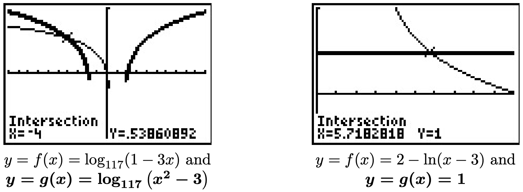
- Since we have the same base on both sides of the equation \(\log_{117}(1-3x) = \log_{117}\left(x^2-3\right)\), we equate what's inside the logs to get \(1-3x = x^2-3\). Solving \(x^2+3x-4 = 0\) gives \(x=-4\) and \(x=1\). To check these answers using the calculator, we make use of the Change of Base Formula and graph \(f(x) = \frac{\ln(1-3x)}{\ln(117)}\) and \(g(x) = \frac{\ln\left(x^2-3\right)}{\ln(117)}\) and we see they intersect only at \(x=-4\). To see what happened to the solution \(x=1\), we substitute it into our original equation to obtain \(\log_{117}(-2) = \log_{117}(-2)\). While these expressions look identical, neither is a real number,1 which means \(x=1\) is not in the domain of the original equation, and is not a solution.
- Our first objective in solving \(2 - \ln(x-3) = 1\) is to isolate the logarithm. We get \(\ln(x-3)=1\), which, as an exponential equation, is \(e^{1} = x-3\). We get our solution \(x=e+3\). On the calculator, we see the graph of \(f(x) = 2 - \ln(x-3)\) intersects the graph of \(g(x) = 1\) at \(x = e+3 \approx 5.718\).
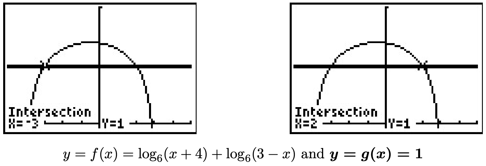
- We can start solving \(\log_{6}(x+4) + \log_{6}(3-x) = 1\) by using the Product Rule for Logarithmic Functions to rewrite the equation as \(\log_{6}\left[(x+4)(3-x)\right] = 1\). Rewriting this as an exponential equation, we get \(6^{1} = (x+4)(3-x)\). This reduces to \(x^2+x-6 = 0\), which gives \(x=-3\) and \(x=2\). Graphing \(y=f(x) = \frac{\ln(x+4)}{\ln(6)} + \frac{\ln(3-x)}{\ln(6)}\) and \(y=g(x) = 1\), we see they intersect twice, at \(x=-3\) and \(x=2\).
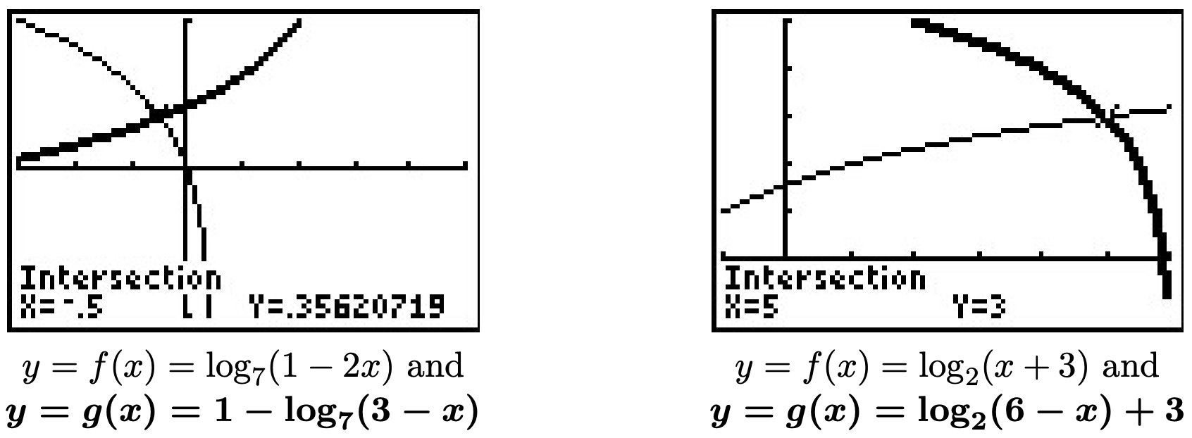
- Taking a cue from the previous problem, we begin solving \(\log_{7}(1-2x) = 1 - \log_{7}(3-x)\) by first collecting the logarithms on the same side, \(\log_{7}(1-2x) + \log_{7}(3-x) = 1\), and then using the Product Rule for Logarithmic Functions to get \(\log_{7}[(1-2x)(3-x)] = 1\). Rewriting this as an exponential equation gives \(7^{1} = (1-2x)(3-x)\) which gives the quadratic equation \(2x^2-7x-4=0\). Solving, we find \(x = -\frac{1}{2}\) and \(x=4\). Graphing, we find \(y = f(x) = \frac{\ln(1-2x)}{\ln(7)}\) and \(y=g(x) = 1 - \frac{\ln(3-x)}{\ln(7)}\) intersect only at \(x=-\frac{1}{2}\). Checking \(x=4\) in the original equation produces \(\log_{7}(-7) = 1 - \log_{7}(-1)\), which is a clear domain violation.
- Starting with \(\log_{2}(x+3) = \log_{2}(6-x)+3\), we gather the logarithms to one side and get \(\log_{2}(x+3) - \log_{2}(6-x) = 3\). We then use the Quotient Rule of Logarithmic Functions and convert to an exponential equation\[\log_{2}\left(\dfrac{x+3}{6-x}\right) = 3 \iff 2^{3} = \dfrac{x+3}{6-x}\nonumber\]This reduces to the linear equation \(8(6-x) = x+3\), which gives us \(x = 5\). When we graph \(f(x) = \frac{\ln(x+3)}{\ln(2)}\) and \(g(x) = \frac{\ln(6-x)}{\ln(2)} + 3\), we find they intersect at \(x=5\).
- Starting with \(1 + 2 \log_{4}(x+1) = 2 \log_{2}(x)\), we gather the logs to one side to get the equation \(1 = 2 \log_{2}(x) - 2 \log_{4}(x+1)\). Before we can combine the logarithms, however, we need a common base. Since \(4\) is a power of \(2\), we use change of base to convert\[\log_{4}(x+1) = \dfrac{\log_{2}(x+1)}{\log_{2}(4)} = \dfrac{1}{2} \log_{2}(x+1)\nonumber\]Hence, our original equation becomes\[\begin{array}{rclcl}
1 & = & 2 \log_{2}(x) - 2 \left(\dfrac{1}{2} \log_{2}(x+1)\right) & & \\[6pt]
1 &= & 2\log_{2}(x) - \log_{2}(x+1) & & \\[6pt]
1 & = & \log_{2}\left(x^2\right) - \log_{2}(x+1) & \quad & \left(\text{Power Rule of Logarithmic Functions}\right) \\[6pt]
1 & = & \log_{2}\left( \dfrac{x^{2}}{x+1}\right) & \quad & \left(\text{Quotient Rule of Logarithmic Functions}\right) \\[6pt]
\end{array}\nonumber\]Rewriting this in exponential form, we get \(\frac{x^{2}}{x+1} = 2\) or \(x^2 -2x-2 = 0\). Using the Quadratic Formula, we get \(x = 1 \pm \sqrt{3}\). Graphing \(f(x) = 1 + \frac{2\ln(x+1)}{\ln(4)}\) and \(g(x) = \frac{2 \ln(x)}{\ln(2)}\), we see the graphs intersect only at \(x = 1 + \sqrt{3} \approx 2.732\). The solution \(x = 1 - \sqrt{3} < 0\), which means if substituted into the original equation, the term \(2 \log_{2}\left(1 - \sqrt{3}\right)\) is undefined.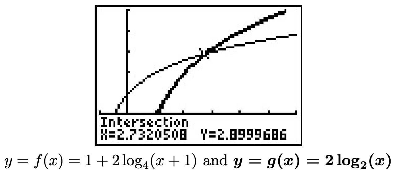
If nothing else, Example \( \PageIndex{1} \) demonstrates the importance of checking for extraneous solutions2 when solving equations involving logarithms. Even though we checked our answers graphically, extraneous solutions are easy to spot - any supposed solution that causes a negative number inside a logarithm must be discarded. As with the equations in Example 6.3.1, much can be learned from analyzing all the answers in Example \( \PageIndex{1} \). We leave this to the reader and focus on inequalities involving logarithmic functions.
Solving Logarithmic Inequalities
Since logarithmic functions are continuous on their domains, we can use sign diagrams.
Solve the following inequalities. Check your answer graphically using a calculator.
- \(\frac{1}{\ln(x)+1} \leq 1\)
- \(\left(\log_{2}(x)\right)^2 < 2 \log_{2}(x) + 3\)
- \(x \log(x+1) \geq x\)
- Solutions
-
- We start solving \(\frac{1}{\ln(x)+1} \leq 1\) by getting \(0\) on one side of the inequality:\[\dfrac{1}{\ln(x)+1} - 1 \leq 0. \nonumber \]Getting a common denominator yields \(\frac{1}{\ln(x)+1} - \frac{\ln(x)+1}{\ln(x)+1} \leq 0\), which reduces to \(\frac{-\ln(x)}{\ln(x)+1} \leq 0\), or\[\dfrac{\ln(x)}{\ln(x)+1} \geq 0. \nonumber \]We define \(r(x) = \frac{\ln(x)}{\ln(x)+1}\) and set about finding the domain and the zeros of \(r\). Due to the appearance of the term \(\ln(x)\), we require \(x > 0\). To keep the denominator away from zero, we solve \(\ln(x)+1 = 0\) so \(\ln(x) = -1\), so \(x = e^{-1} = \frac{1}{e}\). Hence, the domain of \(r\) is\[\left(0, \dfrac{1}{e}\right) \cup \left(\dfrac{1}{e}, \infty\right).\nonumber \]To find the zeros of \(r\), we set \(r(x) = \frac{\ln(x)}{\ln(x)+1} = 0\) so that \(\ln(x) = 0\), and we find \(x = e^{0} = 1\).
To determine test values for \(r\) without resorting to the calculator, we need to find numbers between \(0\), \(\frac{1}{e}\), and \(1\) which have a base of \(e\). Since \(e \approx 2.718 > 1\), \(0 < \frac{1}{e^2} < \frac{1}{e} < \frac{1}{\sqrt{e}} < 1 < e\). To determine the sign of \(r\left( \frac{1}{e^2} \right)\), we use the fact that \(\ln\left(\frac{1}{e^2}\right) = \ln\left(e^{-2}\right) = -2\), and find \(r\left( \frac{1}{e^2} \right) = \frac{-2}{-2+1} = 2\), which is \((+)\). The rest of the test values are determined similarly. From our sign diagram, we find the solution to be \(\left(0, \frac{1}{e}\right) \cup [1, \infty)\).
Graphing \(f(x) = \frac{1}{\ln(x)+1}\) and \(g(x) = 1\), we see the graph of \(f\) is below the graph of \(g\) on the solution intervals, and that the graphs intersect at \(x=1\).
- Moving all of the nonzero terms of \(\left(\log_{2}(x)\right)^2 < 2 \log_{2}(x) + 3\) to one side of the inequality, we have \(\left(\log_{2}(x)\right)^2 - 2 \log_{2}(x) - 3 < 0\). Defining \(r(x) = \left(\log_{2}(x)\right)^2 - 2 \log_{2}(x) - 3\), we get the domain of \(r\) is \((0, \infty)\), due to the presence of the logarithm.
To find the zeros of \(r\), we set \(r(x) =\left(\log_{2}(x)\right)^2 - 2 \log_{2}(x) - 3= 0\) which results in a "quadratic in disguise." We set \(u = \log_{2}(x)\) so our equation becomes \(u^2-2u-3 = 0\) which gives us \(u=-1\) and \(u=3\). Since \(u = \log_{2}(x)\), we get \(\log_{2}(x) = -1\), which gives us \(x = 2^{-1} = \frac{1}{2}\), and \(\log_{2}(x) = 3\), which yields \(x = 2^{3} = 8\).
We use test values which are powers of \(2\): \(0 < \frac{1}{4} < \frac{1}{2} < 1 < 8 < 16\), and from our sign diagram, we see \(r(x)< 0\) on \(\left(\frac{1}{2}, 8 \right)\). Geometrically, we see the graph of \(f(x)= \left(\frac{\ln(x)}{\ln(2)}\right)^2\) is below the graph of \(y = g(x) = \frac{2 \ln(x)}{\ln(2)} + 3\) on the solution interval.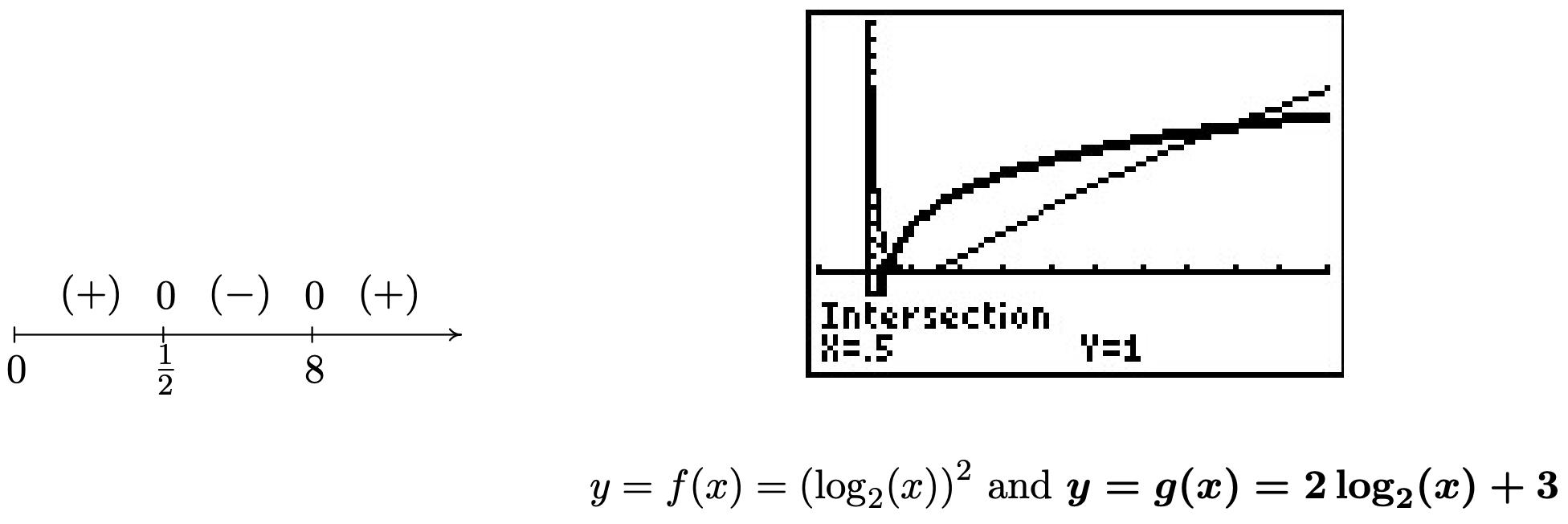
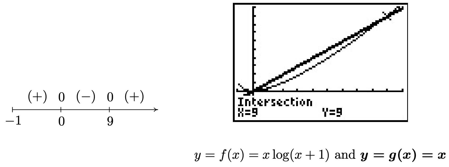
- We begin to solve \(x \log(x+1) \geq x\) by subtracting \(x\) from both sides to get \(x \log(x+1) - x \geq 0\). We define \(r(x) = x \log(x+1) - x\), and due to the presence of the logarithm, we require \(x+1 > 0\), or \(x > -1\). To find the zeros of \(r\), we set \(r(x) = x \log(x+1) - x = 0\). Factoring, we get \(x \left(\log(x+1) - 1\right) = 0\), which gives \(x=0\) or \(\log(x+1) - 1=0\). The latter gives \(\log(x+1) = 1\), or \(x+1 = 10^{1}\), which admits \(x = 9\). We select test values \(x\) so that \(x+1\) is a power of \(10\), and we obtain \(-1 < -0.9 < 0 < \sqrt{10} -1 < 9 < 99\). Our sign diagram gives the solution to be \((-1,0] \cup [9, \infty)\). The calculator indicates the graph of \(y= f(x) = x \log(x+1)\) is above \(y=g(x) = x\) on the solution intervals, and the graphs intersect at \(x=0\) and \(x=9\).
- We start solving \(\frac{1}{\ln(x)+1} \leq 1\) by getting \(0\) on one side of the inequality:\[\dfrac{1}{\ln(x)+1} - 1 \leq 0. \nonumber \]Getting a common denominator yields \(\frac{1}{\ln(x)+1} - \frac{\ln(x)+1}{\ln(x)+1} \leq 0\), which reduces to \(\frac{-\ln(x)}{\ln(x)+1} \leq 0\), or\[\dfrac{\ln(x)}{\ln(x)+1} \geq 0. \nonumber \]We define \(r(x) = \frac{\ln(x)}{\ln(x)+1}\) and set about finding the domain and the zeros of \(r\). Due to the appearance of the term \(\ln(x)\), we require \(x > 0\). To keep the denominator away from zero, we solve \(\ln(x)+1 = 0\) so \(\ln(x) = -1\), so \(x = e^{-1} = \frac{1}{e}\). Hence, the domain of \(r\) is\[\left(0, \dfrac{1}{e}\right) \cup \left(\dfrac{1}{e}, \infty\right).\nonumber \]To find the zeros of \(r\), we set \(r(x) = \frac{\ln(x)}{\ln(x)+1} = 0\) so that \(\ln(x) = 0\), and we find \(x = e^{0} = 1\).
The following example revisits the concept of pH first seen in the homework exercises of Section 6.1.
To successfully breed Ippizuti fish, the pH of a freshwater tank must be at least \(7.8\) but can be no more than \(8.5\). Determine the corresponding range of hydrogen ion concentration, and check your answer using a calculator.
- Solution
-
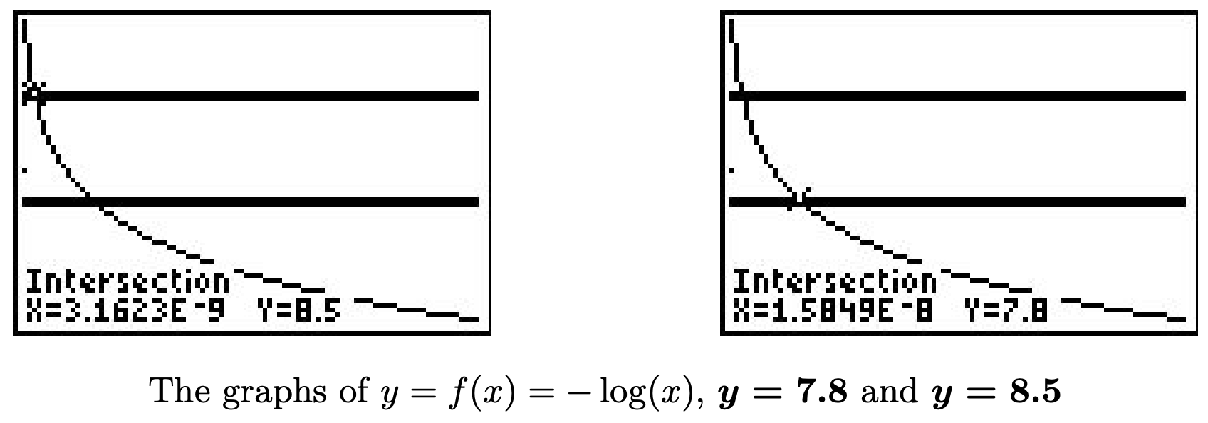
From the homework exercises in Section 6.1, \(\text{pH} = -\log[\text{H}^{+}]\) where \([\text{H}^{+}]\) is the hydrogen ion concentration in moles per liter. We require \(7.8 \leq -\log[\text{H}^{+}] \leq 8.5\) or \(-7.8 \geq \log[\text{H}^{+}] \geq -8.5\). To solve this compound inequality we solve \(-7.8 \geq \log[\text{H}^{+}]\) and \(\log[\text{H}^{+}] \geq -8.5\) and take the intersection of the solution sets.
The former inequality yields \(0 < [\text{H}^{+}] \leq 10^{-7.8}\) and the latter yields \([\text{H}^{+}] \geq 10^{-8.5}\). Taking the intersection gives us our final answer \(10^{-8.5} \leq [\text{H}^{+}] \leq 10^{-7.8}\). (Your Chemistry professor may want the answer written as \(3.16 \times 10^{-9} \leq [\text{H}^{+}] \leq 1.58 \times 10^{-8}\).) After carefully adjusting the viewing window on the graphing calculator, we see that the graph of \(f(x) = -\log(x)\) lies between the lines \(y = 7.8\) and \(y = 8.5\) on the interval \([3.16 \times 10^{-9}, 1.58 \times 10^{-8}]\).
Finding the Inverse When Given an Equation Involving Logarithms
We close this section by finding an inverse of a one-to-one function which involves logarithms.
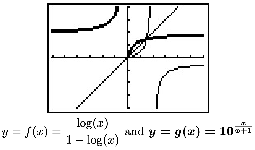
The function \(f(x) = \frac{\log(x)}{1-\log(x)}\) is one-to-one. Find a formula for \(f^{-1}(x)\) and check your answer graphically using your calculator.
- Solution
-
We first write \(y=f(x)\) then interchange the \(x\) and \(y\) and solve for \(y\).\[\begin{array}{rclcl}
y & = & f(x) & & \\[6pt]
y & = & \dfrac{\log(x)}{1-\log(x)} & & \\[6pt]
x & = & \dfrac{\log(y)}{1-\log(y)} & \quad & \left(\text{switching }x\text{ and }y\right)\\[6pt]
x\left(1-\log(y)\right) & = & \log(y) & & \\[6pt]
x - x\log(y) & = & \log(y) & & \\[6pt]
x & = & x \log(y) + \log(y) & & \\[6pt]
x & = & (x+1) \log(y) & & \\[6pt]
\dfrac{x}{x+1} & = & \log(y) & & \\[6pt]
y & = & 10^{\frac{x}{x+1}} & \quad & \left(\text{rewriting as an exponential equation}\right) \\[6pt]
\end{array}\nonumber\]We have \(f^{-1}(x) = 10^{\frac{x}{x+1}}\). Graphing \(f\) and \(f^{-1}\) on the same viewing window yields