
5.5: Harmonic Motion
- Page ID
- 159975

\( \newcommand{\vecs}[1]{\overset { \scriptstyle \rightharpoonup} {\mathbf{#1}} } \)
\( \newcommand{\vecd}[1]{\overset{-\!-\!\rightharpoonup}{\vphantom{a}\smash {#1}}} \)
\( \newcommand{\dsum}{\displaystyle\sum\limits} \)
\( \newcommand{\dint}{\displaystyle\int\limits} \)
\( \newcommand{\dlim}{\displaystyle\lim\limits} \)
\( \newcommand{\id}{\mathrm{id}}\) \( \newcommand{\Span}{\mathrm{span}}\)
( \newcommand{\kernel}{\mathrm{null}\,}\) \( \newcommand{\range}{\mathrm{range}\,}\)
\( \newcommand{\RealPart}{\mathrm{Re}}\) \( \newcommand{\ImaginaryPart}{\mathrm{Im}}\)
\( \newcommand{\Argument}{\mathrm{Arg}}\) \( \newcommand{\norm}[1]{\| #1 \|}\)
\( \newcommand{\inner}[2]{\langle #1, #2 \rangle}\)
\( \newcommand{\Span}{\mathrm{span}}\)
\( \newcommand{\id}{\mathrm{id}}\)
\( \newcommand{\Span}{\mathrm{span}}\)
\( \newcommand{\kernel}{\mathrm{null}\,}\)
\( \newcommand{\range}{\mathrm{range}\,}\)
\( \newcommand{\RealPart}{\mathrm{Re}}\)
\( \newcommand{\ImaginaryPart}{\mathrm{Im}}\)
\( \newcommand{\Argument}{\mathrm{Arg}}\)
\( \newcommand{\norm}[1]{\| #1 \|}\)
\( \newcommand{\inner}[2]{\langle #1, #2 \rangle}\)
\( \newcommand{\Span}{\mathrm{span}}\) \( \newcommand{\AA}{\unicode[.8,0]{x212B}}\)
\( \newcommand{\vectorA}[1]{\vec{#1}} % arrow\)
\( \newcommand{\vectorAt}[1]{\vec{\text{#1}}} % arrow\)
\( \newcommand{\vectorB}[1]{\overset { \scriptstyle \rightharpoonup} {\mathbf{#1}} } \)
\( \newcommand{\vectorC}[1]{\textbf{#1}} \)
\( \newcommand{\vectorD}[1]{\overrightarrow{#1}} \)
\( \newcommand{\vectorDt}[1]{\overrightarrow{\text{#1}}} \)
\( \newcommand{\vectE}[1]{\overset{-\!-\!\rightharpoonup}{\vphantom{a}\smash{\mathbf {#1}}}} \)
\( \newcommand{\vecs}[1]{\overset { \scriptstyle \rightharpoonup} {\mathbf{#1}} } \)
\(\newcommand{\longvect}{\overrightarrow}\)
\( \newcommand{\vecd}[1]{\overset{-\!-\!\rightharpoonup}{\vphantom{a}\smash {#1}}} \)
\(\newcommand{\avec}{\mathbf a}\) \(\newcommand{\bvec}{\mathbf b}\) \(\newcommand{\cvec}{\mathbf c}\) \(\newcommand{\dvec}{\mathbf d}\) \(\newcommand{\dtil}{\widetilde{\mathbf d}}\) \(\newcommand{\evec}{\mathbf e}\) \(\newcommand{\fvec}{\mathbf f}\) \(\newcommand{\nvec}{\mathbf n}\) \(\newcommand{\pvec}{\mathbf p}\) \(\newcommand{\qvec}{\mathbf q}\) \(\newcommand{\svec}{\mathbf s}\) \(\newcommand{\tvec}{\mathbf t}\) \(\newcommand{\uvec}{\mathbf u}\) \(\newcommand{\vvec}{\mathbf v}\) \(\newcommand{\wvec}{\mathbf w}\) \(\newcommand{\xvec}{\mathbf x}\) \(\newcommand{\yvec}{\mathbf y}\) \(\newcommand{\zvec}{\mathbf z}\) \(\newcommand{\rvec}{\mathbf r}\) \(\newcommand{\mvec}{\mathbf m}\) \(\newcommand{\zerovec}{\mathbf 0}\) \(\newcommand{\onevec}{\mathbf 1}\) \(\newcommand{\real}{\mathbb R}\) \(\newcommand{\twovec}[2]{\left[\begin{array}{r}#1 \\ #2 \end{array}\right]}\) \(\newcommand{\ctwovec}[2]{\left[\begin{array}{c}#1 \\ #2 \end{array}\right]}\) \(\newcommand{\threevec}[3]{\left[\begin{array}{r}#1 \\ #2 \\ #3 \end{array}\right]}\) \(\newcommand{\cthreevec}[3]{\left[\begin{array}{c}#1 \\ #2 \\ #3 \end{array}\right]}\) \(\newcommand{\fourvec}[4]{\left[\begin{array}{r}#1 \\ #2 \\ #3 \\ #4 \end{array}\right]}\) \(\newcommand{\cfourvec}[4]{\left[\begin{array}{c}#1 \\ #2 \\ #3 \\ #4 \end{array}\right]}\) \(\newcommand{\fivevec}[5]{\left[\begin{array}{r}#1 \\ #2 \\ #3 \\ #4 \\ #5 \\ \end{array}\right]}\) \(\newcommand{\cfivevec}[5]{\left[\begin{array}{c}#1 \\ #2 \\ #3 \\ #4 \\ #5 \\ \end{array}\right]}\) \(\newcommand{\mattwo}[4]{\left[\begin{array}{rr}#1 \amp #2 \\ #3 \amp #4 \\ \end{array}\right]}\) \(\newcommand{\laspan}[1]{\text{Span}\{#1\}}\) \(\newcommand{\bcal}{\cal B}\) \(\newcommand{\ccal}{\cal C}\) \(\newcommand{\scal}{\cal S}\) \(\newcommand{\wcal}{\cal W}\) \(\newcommand{\ecal}{\cal E}\) \(\newcommand{\coords}[2]{\left\{#1\right\}_{#2}}\) \(\newcommand{\gray}[1]{\color{gray}{#1}}\) \(\newcommand{\lgray}[1]{\color{lightgray}{#1}}\) \(\newcommand{\rank}{\operatorname{rank}}\) \(\newcommand{\row}{\text{Row}}\) \(\newcommand{\col}{\text{Col}}\) \(\renewcommand{\row}{\text{Row}}\) \(\newcommand{\nul}{\text{Nul}}\) \(\newcommand{\var}{\text{Var}}\) \(\newcommand{\corr}{\text{corr}}\) \(\newcommand{\len}[1]{\left|#1\right|}\) \(\newcommand{\bbar}{\overline{\bvec}}\) \(\newcommand{\bhat}{\widehat{\bvec}}\) \(\newcommand{\bperp}{\bvec^\perp}\) \(\newcommand{\xhat}{\widehat{\xvec}}\) \(\newcommand{\vhat}{\widehat{\vvec}}\) \(\newcommand{\uhat}{\widehat{\uvec}}\) \(\newcommand{\what}{\widehat{\wvec}}\) \(\newcommand{\Sighat}{\widehat{\Sigma}}\) \(\newcommand{\lt}{<}\) \(\newcommand{\gt}{>}\) \(\newcommand{\amp}{&}\) \(\definecolor{fillinmathshade}{gray}{0.9}\)The material in this section could easily be taught when covering the material in the previous section. I broke it into its own section because I didn't want to have a massive sinusoidal model section. Also, harmonic motion is a big topic in Differential Equations (nearly a full chapter's worth) and having a single section for it here might make it stand out more for the student.
|
Hawk A.I. Section-Specific Tutor Please note that, to access the Hawk A.I. Tutor, you will need a (free) OpenAI account. |
Harmonic motion is a form of periodic motion, but there are factors to consider that differentiate the two types. Applications involving general periodic motion cycle through their periods with no outside interference. This type of motion is what we have dealt with up to this point in Trigonometry. In terms of sinusoidal functions, we think of this as oscillatory motion.
Examples of oscillatory motion include temperature measurements throughout the day, the elevation of a rider on a Ferris wheel, and sound waves. In all of these examples, the motion is periodic. Still, there is no physical force requiring the measured quantity to tend back to the midline of the periodic motion.
Harmonic motion, on the other hand, requires a restorative force.
As a reminder from Physics, a force can be considered a push or pull. Thus, an object goes through harmonic motion if it oscillates (much like periodic motion) but is constantly being pulled by a force back to the midline of the oscillatory motion. Harmonic motion is crucial in Differential Equations, Engineering, and Physics. Harmonic motion includes the motion of springs, gravitational force, and magnetic force. It can further be broken into two major types - simple harmonic motion (also called undamped harmonic motion) and damped harmonic motion.1
Solving Exponential Equations
The material in this section relies heavily on your knowledge of exponential and logarithmic functions, the Laws of Logarithms, and your ability to solve exponential equations. Since it might have been a while since you have seen such topics, let's take a moment to review the "nuts and bolts" needed for the material at hand.
Many exponential functions appear in population models, where the function values rely on time. Therefore, you will commonly encounter exponential functions in the form \( P(t) = P_0 \cdot b^t \), where \( P(0) = P_0 \cdot b^0 = P_0 \) and, as such, \( P_0 \) is called the initial population.
While there is a chapter's-worth of theory and material we could cover when talking about exponential functions (and the interested student should take a College Algebra course to explore such theory), for this section we just need to recall two pieces of theory. First up is the graph of the exponential function.
An exponential function with the form \( f(x) = b^x \), where \(b > 0\) and \(b \neq 1\), has these characteristics:
- one-to-one function
- horizontal asymptote: \(y=0\)
- domain: \((-\infty , \infty )\)
- range: \((0, \infty )\)
- \( x \)-intercept: none
- \( y \)-intercept: \((0,1)\)
- Secondary key point: \( \left( 1, b \right) \)
- increasing if \(b>1\)
- decreasing if \(0 < b<1\)
The leftmost graph in the theorem above is of significant value when we discuss damped harmonic motion near the end of this section.
The second piece of theory we must recall from Algebra is how to solve a simple exponential equation of the form \( k = e^x \), where \( k \gt 0 \).
To solve such an equation, we need to remember that logarithms and exponentials are inverses to one another. More specifically,\[ \ln\left( e^x \right) = x \quad \text{and} \quad e^{\ln(x)} = x. \nonumber \]Therefore, to solve \( k = e^x \), we apply the natural logarithmic function to both sides of the equation to get the following:\[ \begin{array}{rrcl}
& k & = & e^x \\[6pt] \implies & \ln(k) & = & \ln\left( e^x \right) \\[6pt] \implies & \ln(k) & = & x. \\[6pt] \end{array} \nonumber \]
Simple Harmonic Motion
The "prototype" motion, called simple harmonic motion, involves a restorative force but assumes that the motion will continue forever.
There are two words in this definition that you might be unfamiliar with.
A driven motion is one that experiences an additional pulse of energy. Think of this as the energy a parent gives to a child when they are one a swing. The child's motion on the swing as they go back and forth is harmonic motion. Every once in a while, the parent gives an extra push to the child so that their harmonic motion speeds back up - they are driving the harmonic motion with extra energy (in fact, the child swinging her legs also adds a bit of extra energy to keep her in motion).
In non-driven harmonic motion, the parent would not be pushing the child (and the child would not be swinging her legs to gain more "swing energy"). You can imagine what would happen in this scenario - the swing would oscillate back and forth, but with less magnitude each time. Eventually, the child would stop swinging.
But why would the child stop swinging?
In reality, there is almost always a damping force - a force that slows the oscillatory motion. In the case of the child on the swing, the damping force is due to friction (specifically, the resistive force of friction due to air and likely the friction on the chains connected to the swing set.
Undamped motion, on the other hand, never experiences loss of energy due to friction or other external factors. As such, simple harmonic motion (being both undamped and non-driven) is not the most realistic type of harmonic motion; however, it's a necessary starting point to understand the robust forms.
Imagine a weighted object hanging on a spring. When that object is not disturbed, we say that the object is at rest or in equilibrium. If the object is pulled down and then released, the spring's force (called the spring's restorative force) pulls the object back toward equilibrium, and harmonic motion begins. The restorative force of the spring is directly proportional to the object's displacement from its equilibrium point.2
Observation: The simple harmonic motion of the object is sinusoidal.
The position of a particle relative to the ground is often unimportant when building a model for simple harmonic motion. This is because we are only concerned with modeling the particle's motion - not the height. Moreover, all our previous training with graphs of sinusoidal functions still holds here. The only difference is that we are replacing \( B \) with \( \omega \), and \( C \) with \( \phi \). This is mainly because \( \omega \) and \( \phi \) are the typical notations used in Physics.
Finally, the sinusoidal nature of these phenomena observed in physics is just that - an observation. We have not, and cannot, prove this result in Trigonometry. You do, however, prove this result in Differential Equations.
The displacement of a mass suspended by a spring is modeled by the function\[ s(t) = 1.5\sin\left( 6\pi t \right), \nonumber \]where \( s(t) \) is measured in cm and \( t \) in seconds.
- Find the amplitude, period, and frequency of the motion of the mass.
- Sketch a graph of the displacement of the mass.
- Solutions
-
- From our previous experience, the amplitude is \( |1.5| = 1.5 \), the period is \( \frac{2\pi}{\omega} = \frac{2\pi}{6\pi} = \frac{1}{3} \) seconds per cycle, and the frequency is \( f = \frac{1}{\text{Period}} = 3 \) cycles per second.
-
Figure \( \PageIndex{ 1 } \) 

A mass suspended from a spring is pulled 3 cm below its resting position. The mass is released at time \(t=0\) and allowed to oscillate. After \(\frac{1}{3}\) second, it is observed that the mass returns to its lowest position. Find a function to model this motion relative to its initial resting position.
- Answer
-
\(s(t)=-3 \cos \left(6 \pi t\right)\)
Damped Harmonic Motion
In reality, a pendulum does not swing back and forth forever, and an object on a spring does not bounce up and down forever. Eventually, the pendulum stops swinging, the object stops bouncing, and both return to equilibrium. As mentioned previously, periodic motion in which a damping force (typically friction) acts is known as damped harmonic motion.
Observation: The quasi-sinusoidal harmonic motion of the object is being damped.
In Physics, various formulas account for the damping factor on the moving object. Some of these are Calculus-based formulas that involve derivatives. We will use damping functions based on decreasing exponential functions (as these are the most common damping functions).
The words quasi-period and quasi-frequency reflect the fact that these models are not true sinusoidal models.
Conceptually (and graphically), the decreasing exponential function forces a boundary on the model's position values (outputs). The following Interactive Element should provide more understanding than I could write in a few paragraphs.
Interact: Move the slider to adjust the damping factor.
Observation: The boundary of the damped harmonic motion is always \( y = \pm A \, e^{-c t} \).
Model the equations that fit the two scenarios and use graphing technology to graph the functions: Two mass-spring systems exhibit damped harmonic motion at a quasi-frequency of 0.5 cycles per second. Both have an initial displacement of 10 cm. The first has a damping factor of 0.5, and the second has a damping factor of 0.1.
- Solutions
-
At time \(t=0\), the displacement is the maximum of 10 cm, which calls for the cosine function. The cosine function will apply to both models. We are given the quasi-frequency, \(f=\frac{\omega}{2\pi}\), of 0.5 cycles per second. Thus,\[\begin{array}{rrcl}
& \dfrac{\omega}{2\pi} & = & 0.5 \\[6pt] \implies & \omega & = & \pi \\[6pt] \end{array} \nonumber \]The first spring system has a damping factor of \(c=0.5\). Following the general model for damped harmonic motion, we have\[s_1(t)=10e^{−0.5t} \cos (\pi t). \nonumber\]Figure \( \PageIndex{ 2 } \) 
The second spring system has a damping factor of \(c=0.1\) and can be modeled as\[s_2(t)=10e^{−0.1t} \cos (\pi t).\nonumber \]
Figure \( \PageIndex{ 3 } \) 
Notice the differing effects of the damping constant. The function's local maximum and minimum values with the damping factor \(c=0.5\) decrease much more rapidly than the function with \(c=0.1\).


Find and graph a function of the form \(s(t)=A \, e^{−ct} \cos\left( \omega t \right)\) that models the information given.
- \(A=20, \, c=0.05,\) and the quasi-period is \(4\)
- \(A=2, \, c=1.5,\) and the quasi-frequency is \(3\)
- Answers
-
- \(s(t)=20e^{−0.05t} \cos \left(\frac{\pi}{2}t\right).\)
Figure \( \PageIndex{ 4 } \) 
- \(s(t)=2e^{−1.5t} \cos \left(6\pi t\right).\)
Figure \( \PageIndex{ 5 } \) 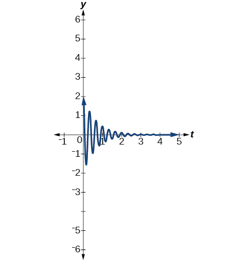
- \(s(t)=20e^{−0.05t} \cos \left(\frac{\pi}{2}t\right).\)
Find and graph a function of the form \(s(t) = A \, e^{−ct} \sin\left( \omega t \right)\) that models the information given.
- \(A=7\), \(c=10\), and the quasi-period is \(p = \frac{\pi}{6}\)
- \(A=0.3\), \(c=0.2\), and the quasi-frequency is \(f=20\)
- Solutions
-
Calculate the value of \(\omega\) and substitute the known values into the model.
- As the quasi-period is \(\frac{2\pi}{\omega}\), we have\[\begin{array}{rrcl}
& \dfrac{\pi}{6} & = & \dfrac{2\pi}{\omega} \\[6pt] \implies & \omega \pi & = & 6(2 \pi) \\[6pt] \implies & \omega & = & 12 \\[6pt] \end{array} \nonumber \]The damping factor is given as 10 and \( A \) is 7. Thus, the model is \(s(t)=7e^{−10t} \sin (12t)\).Figure \( \PageIndex{ 6 } \) 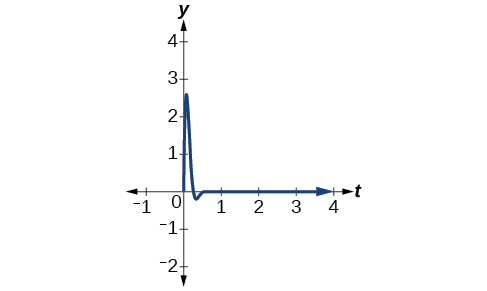
- As the quasi-frequency is \(\frac{\omega}{2\pi}\), we have\[\begin{array}{rrcl}
& 20 & = & \dfrac{\omega}{2\pi} \\[6pt] \implies & 40\pi & = & \omega \\[6pt] \end{array} \nonumber \]The damping factor is given as \(0.2\) and \(A = 0.3\). The model is \(s(t)=0.3e^{−0.2t} \sin (40\pi t)\).Figure \( \PageIndex{ 7 } \) 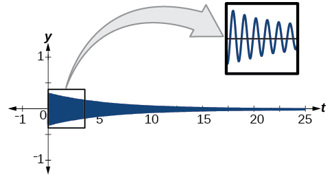
- As the quasi-period is \(\frac{2\pi}{\omega}\), we have\[\begin{array}{rrcl}
A comparison of Examples \( \PageIndex{ 3a } \) and \( \PageIndex{ 3b } \) illustrates how we choose between the sine or cosine functions to model sinusoidal criteria. We see that the cosine function is at the maximum displacement when \(t=0\), and the sine function is at the equilibrium point when \(t=0.\) For example, consider the equation\[y=20e^{−0.05t} \cos\left(\dfrac{\pi}{2}t\right)\nonumber \]from Checkpoint \( \PageIndex{ 2 } \). We can see from the graph that when \(t=0\), \(y=20\), which is the initial amplitude. Check this by setting \(t=0\) in the cosine equation:\[ \begin{array}{rcl}
y & = & 20e^{−0.05(0)} \cos\left(\dfrac{\pi}{2} \cdot 0\right) \\[6pt] & = & 20(1)(1) \\[6pt] & = & 20 \\[6pt] \end{array}\nonumber \]Using the sine function yields\[\begin{array}{rcl}
y & = & 20e^{−0.05(0)} \sin\left(\dfrac{\pi}{2} \cdot 0\right) \\[6pt] & = & 20(1)(0) \\[6pt] & = & 0 \\[6pt] \end{array}\nonumber \]Thus, cosine is the correct function.
Write the equation for damped harmonic motion given \(A=10\), \(c=0.5\), and the quasi-period is \(p=2\), where the initial value of the function is \( s(0) = -10 \).
- Answer
-
\(s(t)=-10e^{−0.5t} \cos (\pi t)\)
A spring measuring 10 inches in natural length is compressed by 5 inches and released. It oscillates once every 3 seconds, and its amplitude decreases by 30% every second. Find an equation that models the position of the spring \(t\) seconds after being released.
- Solution
-
The amplitude begins at 5 inches and deceases by 30% each second. We will make an "amplitude function" as an intermediate step. We can write the amplitude portion of the function as\[\text{Amp}(t) = A e^{-ct}. \nonumber\]We know that the amplitude is 5 when \( t = 0 \). Hence,\[ 5 = Ae^{-c(0)} \implies 5 = Ae^{0} \implies 5 = A (1) \implies 5 = A. \nonumber \]Therefore, our amplitude function becomes\[ \text{Amp}(t) = 5e^{-ct}. \nonumber \]We also know the amplitude drops by 30% when \( t = 1 \). "Dropping by 30%" is the same as saying the amplitude at \( t = 1 \) is 70% (100% minus 30%) of its original value at \( t = 1 \). Thus, we want to solve \( 0.7(5) = 5e^{-c(1)} \).\[\begin{array}{rrclcl}
& 0.7(5) & = & 5e^{-c(1)} & & \\[6pt] \implies & 0.7 & = & e^{-c} & \quad & \left( \text{dividing} \right) \\[6pt] \implies & \ln\left( 0.7 \right) & = & -c & \quad & \left( \text{taking the log of both sides} \right) \\[6pt] \implies & -\ln\left( 0.7 \right) & = & c & \quad & \left( \text{solving for }c \right) \\[6pt] \implies & c & \approx & −0.357 & & \\[6pt] \end{array} \nonumber \]Let’s address the quasi-period. The spring completes a cycle every 3 seconds. This is the quasi-period, and we can use the formula to find \(\omega\).\[\begin{array}{rrcl}
& 3 & = & \dfrac{2 \pi }{\omega} \\[6pt]
\implies & \omega & = & \dfrac{2 \pi }{3} \\[6pt]
\end{array} \nonumber \]The natural length of 10 inches is the midline. We will use the cosine function since the spring starts at maximum displacement. This portion of the equation is represented as\[y = \cos \left(\dfrac{2 \pi }{3}t\right)+10. \nonumber\]Finally, we put both functions together. Our model for the position of the spring at \(t\) seconds is given as\[y \approx 5e^{−0.357t} \cos \left(\dfrac{2 \pi }{3}t\right)+10. \nonumber\]The approximation sign is needed because the coefficient of \( t \) is an approximation.Figure \( \PageIndex{ 8 } \) 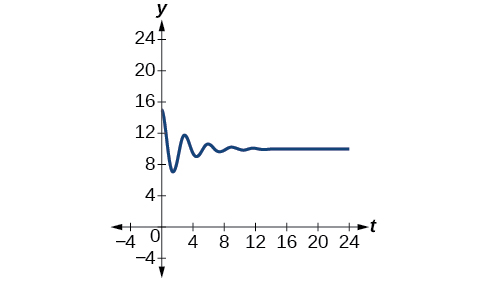
A guitar string is plucked and vibrates in a damped harmonic motion. The string is pulled and displaced 2 cm from its resting position. After 3 seconds, the displacement measures 1 cm. Find the damping constant.
- Solution
-
Following our tactic from Example \( \PageIndex{ 4 } \), we recognize that the initial displacement, 2 cm, represents \( A \). Therefore, the amplitude function for our model is\[ \text{Amp}(t) = 2e^{-ct}. \nonumber \]It is stated that after 3 seconds, maximum displacement measures one-half of its original value. Therefore, we have the equation\[ \dfrac{2}{2} = 3 \, e^{−c(3)}.\nonumber \]Solving for \(c\), we get the following:\[\begin{array}{rrclcl}
& \dfrac{2}{2} & = & 2 \, e^{−c(3)} & & \\[6pt]
\implies & 1 & = & 2 e^{−3c} & \quad & \left( \text{simplifying} \right) \\[6pt]
\implies & \dfrac{1}{2} & = & e^{−3c} & \quad & \left( \text{dividing both sides by }2 \right) \\[6pt]
\implies & \ln\left(\dfrac{1}{2}\right) & = & −3c & \quad & \left( \text{taking the ln of both sides} \right) \\[6pt]
\implies & -\dfrac{\ln\left(\frac{1}{2}\right)}{3} & = & c & \quad & \left( \text{dividing both sides by }-3 \right) \\[6pt]
\implies & \dfrac{\ln\left(\frac{1}{2}\right)^{-1}}{3} & = & c & \quad & \left( \text{Laws of Logarithms} \right) \\[6pt]
\implies & \dfrac{\ln(2)}{3} & = & c & \quad & \left( \text{Laws of Exponents} \right) \\[6pt]
\end{array}\nonumber \]Thus, the damping constant is \(c = \frac{\ln(2)}{3}\).
Footnotes
1 Within both simple and damped harmonic motion, you also encounter free and driven (or forced) motion. These topics are reserved for Differential Equations; however, you can think of free motion as motion without extra external forces being applied. Driven (or forced) motion occurs when the object gains or loses kinetic energy due to an extra external force being applied.
For example, if we attach a mass to a spring, allow it to stretch to equilibrium, pull down slightly once it has reached equilibrium, and then let go, the motion of the mass will be free, damped motion. It starts oscillating, and we do not add any other forces to its movement; however, the spring constantly tries to pull (or push) the mass back to equilibrium. As time goes on, the amplitude of the oscillations decreases as the mass settles to the equilibrium position.
On the other hand, if we attach a mass to a spring, allow it to stretch to equilibrium, pull down slightly once it has reached equilibrium, let go, and then give it an extra push each time it reaches its lowest point (kind of like pushing a child on a swing), the motion is driven, damped motion. It's still damped because we are trying to be realistic by assuming that, when left alone, the amplitude of the oscillations should get smaller; however, it is driven because we add energy to the mass by pushing it each time it reaches its lowest point.
2 From Algebra, \( F \) is directly proportional to \( x \) if there exists a constant, \( k \), such that \( F = k x \). \( k \) is called the constant of proportionality.