7.6: Modeling with Trigonometric Equations

Determining the Amplitude and Period of a Sinusoidal Function

Any motion that repeats itself in a fixed time period is considered periodic motion and can be modeled by a sinusoidal function. The amplitude of a sinusoidal function is the distance from the midline to the maximum value, or from the midline to the minimum value. The midline is the average value. Sinusoidal functions oscillate above and below the midline, are periodic, and repeat values in set cycles. Recall from Graphs of the Sine and Cosine Functions that the period of the sine function and the cosine function is \(2π\). In other words, for any value of \(x\),

\[ \sin(x±2πk)=\sin x \; \text{and} \; \cos(x±2πk)=\cos x \]

where \(k\) is an integer.

STANDARD FORM OF SINUSOIDAL EQUATIONS

The general forms of a sinusoidal equation are given as

\[y=A \sin(Bt−C)+D\]

or

\[ y=A \cos(Bt−C)+D\]

where \(\text{amplitude}=|A|,B\) is related to period such that the \(\text{period}=\frac{2π}{B},C\) is the phase shift such that \(\frac{C}{B}\) denotes the horizontal shift, and \(D\) represents the vertical shift from the graph’s parent graph.

Note that the models are sometimes written as

\[y=a \sin (ω t±C)+D\]

or

\[y=a \cos(ω t±C)+D,\]

with a period that is given as \(\frac{2π}{ω}\).

The difference between the sine and the cosine graphs is that the sine graph begins with the average value of the function and the cosine graph begins with the maximum or minimum value of the function.

Example \(\PageIndex{1}\): Showing How the Properties of a Trigonometric Function Can Transform a Graph

Show the transformation of the graph of \(y=\sin x\) into the graph of \(y=2 \sin(4x−\frac{π}{2})+2\).

Solution

Consider the series of graphs in Figure \(\PageIndex{1}\) and the way each change to the equation changes the image.

Figure \(\PageIndex{2}\):

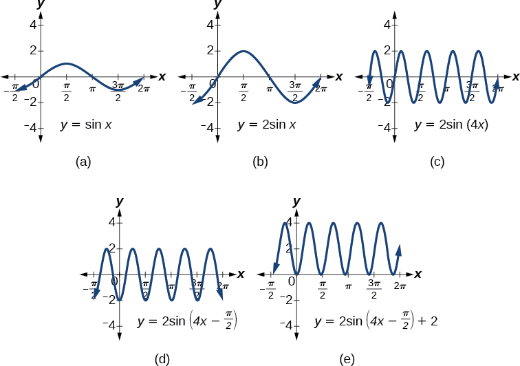
1. The basic graph of \(y=\sin x\)
2. Changing the amplitude from 1 to 2 generates the graph of \(y=2 \sin x\).
3. The period of the sine function changes with the value of \(B,\) such that \(\text{period}=\frac{2π}{B}.\) Here we have \(B=4,\) which translates to a period of \(\frac{π}{2}\). The graph completes one full cycle in \(\frac{π}{2}\) units.
4. The graph displays a horizontal shift equal to \(\frac{C}{B}\), or \(\frac{\frac{π}{2}}{4}=\frac{π}{8}\).
5. Finally, the graph is shifted vertically by the value of \(D\). In this case, the graph is shifted up by 2 units.

Modeling Periodic Behavior

We will now apply these ideas to problems involving periodic behavior.

Example \(\PageIndex{4}\): Modeling an Equation and Sketching a Sinusoidal Graph to Fit Criteria

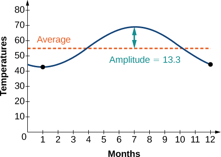
The average monthly temperatures for a small town in Oregon are given in Table \(\PageIndex{1}\). Find a sinusoidal function of the form \(y=A \sin (Bt−C)+D\) that fits the data (round to the nearest tenth) and sketch the graph.

Table \(\PageIndex{2}\)

Month	Temperature,\(^oF\)
January	42.5
February	44.5
March	48.5
April	52.5
May	58
June	63
July	68.5
August	69
September	64.5
October	55.5
November	46.5
December	43.5

Solution

Recall that amplitude is found using the formula

\[A=\dfrac{\text{largest value −smallest value}}{2}\]

Thus, the amplitude is

\[\begin{align*} |A| & = \dfrac{69−42.5}{2} \\ &=13.25 \end{align*}\]

The data covers a period of 12 months, so \(\frac{2π}{B}=12\) which gives \(B=\frac{2π}{12}=\frac{π}{6}\).

The vertical shift is found using the following equation.

\[D=\dfrac{\text{highest value+lowest value}}{2}\]

Thus, the vertical shift is

\[\begin{align*} D &= \dfrac{69+42.5}{2} &=55.8 \end{align*}\]

So far, we have the equation \(y=13.3 \sin (\frac{π}{6}x−C)+55.8\).

To find the horizontal shift, we input the \(x\) and \(y\) values for the first month and solve for \(C\).

\[\begin{align*} 42.5 & =13.3 \sin (\frac{π}{6}(1)−C)+55.8 \\ −13.3 & =13.3 \sin (\frac{π}{6}−C) \\ −1 & =\sin (\frac{π}{6}−C) \;\;\;\;\;\;\;\; \sin θ=−1→ θ=−\frac{π}{2} \\ \frac{π}{6}−C=−\frac{π}{2} \\ \frac{π}{6}+\frac{π}{2} & =C \\ &=\frac{2π}{3} \end{align*}\]

We have the equation \(y=13.3 \sin (\frac{π}{6}x−\frac{2π}{3})+55.8\). See the graph in Figure \(\PageIndex{9}\).

Figure \(\PageIndex{9}\)

Modeling Harmonic Motion Functions

Harmonic motion is a form of periodic motion, but there are factors to consider that differentiate the two types. While general periodic motion applications cycle through their periods with no outside interference, harmonic motion requires a restoring force. Examples of harmonic motion include springs, gravitational force, and magnetic force.

Simple Harmonic Motion

A type of motion described as simple harmonic motion involves a restoring force but assumes that the motion will continue forever. Imagine a weighted object hanging on a spring, When that object is not disturbed, we say that the object is at rest, or in equilibrium. If the object is pulled down and then released, the force of the spring pulls the object back toward equilibrium and harmonic motion begins. The restoring force is directly proportional to the displacement of the object from its equilibrium point. When \(t=0,d=0.\)

SIMPLE HARMONIC MOTION

We see that simple harmonic motion equations are given in terms of displacement:

\[d=a \cos (ωt) \; \text{or} \; d=a \sin (ωt) \]

where \(| a |\) is the amplitude, \(\frac{2π}{ω}\) is the period, and \(\frac{ω}{2π}\) is the frequency, or the number of cycles per unit of time.

Exercise \(\PageIndex{5}\): Finding the Displacement, Period, and Frequency, and Graphing a Function

For each the given functions:

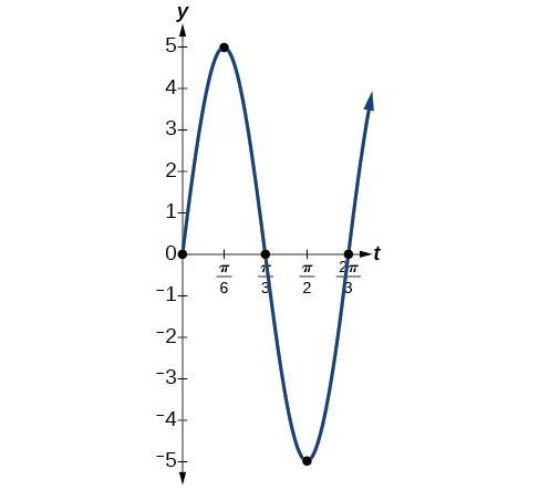
1. \(y=5 \sin (3t)\)
2. \(y=6 \cos (πt)\)
3. \(y=5 \cos (\frac{π}{2}) t\)

address the following questions:

1. Find the maximum displacement of an object.
2. Find the period or the time required for one vibration.
3. Find the frequency.
4. Sketch the graph.

Figure \(\PageIndex{13}\)

Answer a

1. The maximum displacement is equal to the amplitude,\( |a|\), which is 5.
2. The period is \(\frac{2π}{ω}=\frac{2π}{3}\).
3. The frequency is given as \(\frac{ω}{2π}=\frac{3}{2π}\).
4. See Figure \(\PageIndex{13}\). The graph indicates the five key points.

Answer b

1. The maximum displacement is \(6\).
2. The period is \(\frac{2π}{ω}=\frac{2π}{π}=2.\)
3. The frequency is \(\frac{ω}{2π}=\frac{π}{2π}=\frac{1}{2}.\)
4. See Figure \(\PageIndex{14}\).

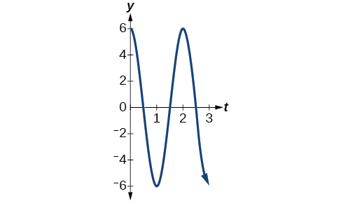
Figure \(\PageIndex{14}\)

Answer c

1. The maximum displacement is \(5\).
2. The period is \(\frac{2π}{ω}=\frac{2π}{\frac{π}{2}}=4\).
3. The frequency is \(\frac{1}{4}.\)
4. See Figure \(\PageIndex{15}\).

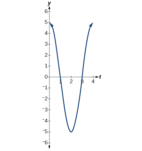
Figure \(\PageIndex{15}\)

Damped Harmonic Motion

In reality, a pendulum does not swing back and forth forever, nor does an object on a spring bounce up and down forever. Eventually, the pendulum stops swinging and the object stops bouncing and both return to equilibrium. Periodic motion in which an energy-dissipating force, or damping factor, acts is known as damped harmonic motion. Friction is typically the damping factor.

In physics, various formulas are used to account for the damping factor on the moving object. Some of these are calculus-based formulas that involve derivatives. For our purposes, we will use formulas for basic damped harmonic motion models.

Definition: DAMPED HARMONIC MOTION

In damped harmonic motion, the displacement of an oscillating object from its rest position at time \(t\) is given as

\[ f(t)=ae^{−ct} \sin (ωt) \; \text{ or} \; f(t)=ae^{−ct} \cos (ωt)\]

where \(c\) is a damping factor, \(|a|\) is the initial displacement and \(\frac{2π}{ω}\) is the period.

Example \(\PageIndex{8}\): Modeling Damped Harmonic Motion

Model the equations that fit the two scenarios and use a graphing utility to graph the functions: Two mass-spring systems exhibit damped harmonic motion at a frequency of 0.5 cycles per second. Both have an initial displacement of 10 cm. The first has a damping factor of 0.5 and the second has a damping factor of 0.1.

Solution

At time \(t=0\), the displacement is the maximum of 10 cm, which calls for the cosine function. The cosine function will apply to both models.

We are given the frequency \(f=\frac{ω}{2π}\) of 0.5 cycles per second. Thus,

\[\begin{align*} \dfrac{ω}{2π} &=0.5 \\ ω&=(0.5)2π \\ &=π \end{align*}\]

The first spring system has a damping factor of \(c=0.5\). Following the general model for damped harmonic motion, we have

\[f(t)=10e^{−0.5t} \cos (πt) \nonumber\]

Figure \(\PageIndex{16}\) models the motion of the first spring system.

Figure \(\PageIndex{16}\)

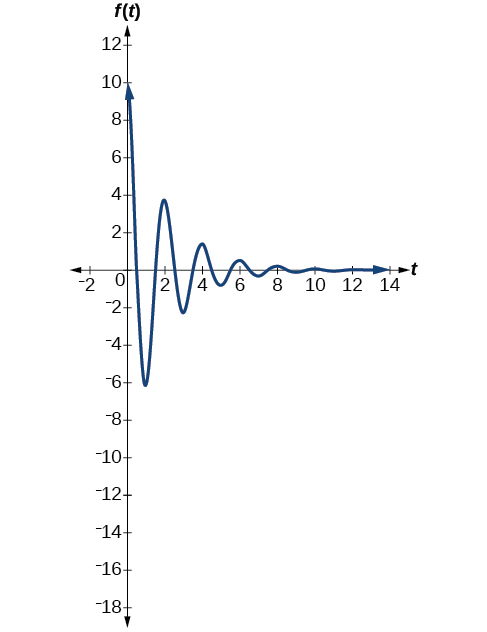
The second spring system has a damping factor of \(c=0.1\) and can be modeled as

\[f(t)=10e^{−0.1t} \cos (πt)\]

Figure \(\PageIndex{17}\) models the motion of the second spring system.

Figure \(\PageIndex{17}\)

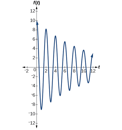
Analysis

Notice the differing effects of the damping constant. The local maximum and minimum values of the function with the damping factor \(c=0.5\) decreases much more rapidly than that of the function with \(c=0.1\).

Bounding Curves in Harmonic Motion

Harmonic motion graphs may be enclosed by bounding curves. When a function has a varying amplitude, such that the amplitude rises and falls multiple times within a period, we can determine the bounding curves from part of the function.

Example \(\PageIndex{12}\): Graphing an Oscillating Cosine Curve

Graph the function \(f(x)=\cos (2πx) \cos (16πx)\).

Solution

The graph produced by this function will be shown in two parts. The first graph will be the exact function \(f(x)\) (see Figure \(\PageIndex{23; top}\);), and the second graph is the exact function \(f(x)\) plus a bounding function (see Figure \(\PageIndex{23; bottom}\)). The graphs look quite different.

Figure_07_07_016.jpg" />

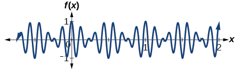
Figure \(\PageIndex{23}\)

Analysis

The curves \(y=\cos (2πx)\) and \(y=−\cos (2πx)\) are bounding curves: they bound the function from above and below, tracing out the high and low points. The harmonic motion graph sits inside the bounding curves. This is an example of a function whose amplitude not only decreases with time, but actually increases and decreases multiple times within a period.