15.2: The Hyperbola

Learning Objectives Locate a hyperbola’s vertices and foci. Write equations of hyperbolas in standard form. Graph hyperbolas centered at the origin. Graph hyperbolas not centered at the origin. Solve applied problems involving hyperbolas.

Hawk A.I. Section-Specific Tutor Please note that, to access the Hawk A.I. Tutor, you will need a (free) OpenAI account.

What do paths of comets, supersonic booms, ancient Grecian pillars, and natural draft cooling towers have in common? They can all be modeled by the same type of conic. For instance, when something moves faster than the speed of sound, a shock wave in the form of a cone is created. A portion of a conic is formed when the wave intersects the ground, resulting in a sonic boom. See Figure \( \PageIndex{ 1 } \).

Figure \( \PageIndex{ 1 } \)

A shock wave intersecting the ground forms a portion of a conic and results in a sonic boom.
 

Most people are familiar with the sonic boom created by supersonic aircraft, but humans were breaking the sound barrier long before the first supersonic flight. The crack of a whip occurs because the tip is exceeding the speed of sound. The bullets shot from many firearms also break the sound barrier, although the bang of the gun usually supersedes the sound of the sonic boom.

Hyperbolas as Conic Sections

In analytic Geometry, a hyperbola is a conic section formed by intersecting a right circular cone with a plane at an angle such that both halves of the cone are intersected. This intersection produces two separate unbounded curves that are mirror images of each other. See Figure \( \PageIndex{ 2 } \).

Figure \( \PageIndex{ 2 } \)

A hyperbola
 

Like the ellipse, the hyperbola can also be defined as a set of points in the coordinate plane.

Definition: Hyperbola

A hyperbola is the set of all points in a plane such that the difference of the distances between the point and two fixed points is a positive constant. Each fixed point is called a focus (plural: foci).

Notice that the definition of a hyperbola is very similar to that of an ellipse. The distinction is that the hyperbola is defined in terms of the difference of two distances, whereas the ellipse is defined in terms of the sum of two distances.

As with the ellipse, every hyperbola has two axes of symmetry and several key points.

Definition: Transverse and Conjugate Axes, Vertex and Co-Vertex, and Center of a Hyperbola

The line segment that passes through the center of the hyperbola and has vertices as its endpoints is called transverse axis. The conjugate axis is perpendicular to the transverse axis and has the co-vertices as its endpoints. The center of the hyperbola is the midpoint of both the transverse and conjugate axes.

Students often think of the transverse axis of a hyperbola as analogous to the major axis for an ellipse. Likewise, they consider conjugate axis of a hyperbola as analogous to the minor axis.

Every hyperbola also has two asymptotes that pass through its center. As a hyperbola recedes from the center, its branches approach these asymptotes. The central rectangle of the hyperbola is centered at the center of the hyperbola with sides that pass through each vertex and co-vertex; it is a useful tool for graphing the hyperbola and its asymptotes. To sketch the asymptotes of the hyperbola, simply sketch and extend the diagonals of the central rectangle. See Figure \( \PageIndex{ 3 } \).

Figure \( \PageIndex{ 3 } \)

Key features of the hyperbola
 

As we did with ellipses, we limit our discussion to hyperbolas that are positioned vertically or horizontally in the coordinate plane; the axes will either lie on or be parallel to the \( x \)- and \( y \)-axes. We will consider two cases: those that are centered at the origin, and those that are centered at a point other than the origin.

Standard Form of a Hyperbola Centered at the Origin

Theorem: Standard Form of the Equation of a Hyperbola Centered at the Origin

The standard form of the equation of a hyperbola with center \((0,0)\) and transverse axis on the \(x\)-axis is\[\dfrac{x^2}{v_x^2}-\dfrac{y^2}{v_y^2}=1, \nonumber \]where

• \( v_x \) and \( v_y \) are positive
• the length of the transverse axis is \(2 v_x\)
• the coordinates of the vertices are \(( \pm v_x, 0)\)
• the length of the conjugate axis is \(2 v_y\)
• the coordinates of the co-vertices are \((0, \pm v_y)\)
• the coordinates of the foci are \(( \pm c, 0)\), where \(c^2= \left| v_x^2 + v_y^2 \right| \)
• the equations of the asymptotes are \( y = \pm \frac{v_y}{v_x} x \).

The standard form of the equation of a hyperbola with center \((0,0)\) and transverse axis on the \(y\)-axis is\[ \dfrac{y^2}{v_y^2}-\dfrac{x^2}{v_x^2}=1, \nonumber \]where

• \( v_x \) and \( v_y \) are positive
• the length of the transverse axis is \(2 v_y\)
• the coordinates of the vertices are \((0, \pm v_y)\)
• the length of the conjugate axis is \(2 v_x\)
• the coordinates of the co-vertices are \(( \pm v_x, 0)\)
• the coordinates of the foci are \((0, \pm c)\), where \(c^2 = \left| v_x^2 + v_y^2 \right| \)
• the equations of the asymptotes are \( y = \pm \frac{v_y}{v_x} x \).

Proof

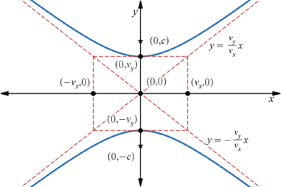
To derive the equation of a hyperbola centered at the origin, we begin with the foci \( (−c,0) \) and \( (c,0) \). The hyperbola is the set of all points \( (x,y) \) such that the difference of the distances from \( (x,y) \) to the foci is constant, as shown in the figure below.

If \((v_x, 0)\) is a vertex of the hyperbola (on the transverse axis), the distance from \((-c, 0)\) to \((v_x, 0)\) is \(v_x-(-c)=v_x+c\). The distance from \((c, 0)\) to \((v_x, 0)\) is \(c - v_x\) (this is where the difference in the proof between the ellipse and the hyperbola begin to differ - notice from the figure above that \( c > v_x \)). The difference of the distances from the foci to the vertex is\[(v_x+c)-(c - v_x) = 2v_x. \nonumber \]If \((x, y)\) is a point on the hyperbola, then we can define the following variables:\[ \begin{array}{rcl} d_1 & = & \text { the distance from }(-c, 0) \text { to }(x, y) \\[6pt] d_2 & = & \text { the distance from }(c, 0) \text { to }(x, y)\\[6pt] \end{array} \nonumber \]By the definition of a hyperbola, \(d_1- d_2\) is constant for any point \((x, y)\) on the hyperbola. We know that the difference of these distances is \(2 v_x\) for the vertex \((v_x, 0)\). It follows that \(d_1-d_2=2 v_x\) for any point on the hyperbola. We will begin the derivation by applying the Distance Formula. The rest of the derivation is algebraic.\[ \begin{array}{rrclcl}
& d_1 - d_2 & = & 2v_x & & \\[6pt]
\implies & \sqrt{\left( x - (-c) \right)^2 + \left( y - 0 \right)^2} - \sqrt{\left( x - c \right)^2 + \left( y - 0 \right)^2} & = & 2v_x & \quad & \left( \text{substituting} \right) \\[6pt]
\implies & \sqrt{\left( x + c \right)^2 + y^2} - \sqrt{\left( x - c \right)^2 + y^2} & = & 2v_x & \quad & \left( \text{simplifying} \right) \\[6pt]
\implies & \sqrt{\left( x + c \right)^2 + y^2} & = & 2v_x + \sqrt{\left( x - c \right)^2 + y^2} & \quad & \left( \text{isolating a radical} \right) \\[6pt]
\implies & \left( x + c \right)^2 + y^2 & = & \left[ 2v_x + \sqrt{\left( x - c \right)^2 + y^2} \right]^2 & \quad & \left( \text{squaring both sides} \right) \\[6pt]
\implies & \left( x + c \right)^2 + y^2 & = & 4v_x^2 + 4v_x \sqrt{\left( x - c \right)^2 + y^2} + \left( x - c \right)^2 + y^2 & \quad & \left( \text{distributing} \right) \\[6pt]
\implies & x^2 + 2 c x + c^2 + y^2 & = & 4v_x^2 + 4v_x \sqrt{\left( x - c \right)^2 + y^2} + x^2 - 2c x + c^2 + y^2 & \quad & \left( \text{distributing} \right) \\[6pt]
\implies & 2 c x & = & 4v_x^2 + 4v_x \sqrt{\left( x - c \right)^2 + y^2} - 2c x & \quad & \left( \text{subtracting }x^2, \, c^2, \text{ and }y^2 \right. \\[6pt]
 &  &  & & \quad & \left. \text{ from both sides} \right) \\[6pt]
\implies & 4 c x - 4v_x^2 & = & 4v_x \sqrt{\left( x - c \right)^2 + y^2} & \quad & \left( \text{isolating the radical} \right) \\[6pt]
\implies & c x - v_x^2 & = & v_x \sqrt{\left( x - c \right)^2 + y^2} & \quad & \left( \text{dividing both sides by }4 \right) \\[6pt]
\implies & \left(c x - v_x^2\right)^2 & = & v_x^2 \left(\left( x - c \right)^2 + y^2\right) & \quad & \left( \text{squaring both sides} \right) \\[6pt]
\implies & c^2 x^2 - 2v_x^2 c x + v_x^4 & = & v_x^2 \left(x^2 - 2cx + c^2 + y^2\right) & \quad & \left( \text{distributing} \right) \\[6pt]
\implies & c^2 x^2 - 2v_x^2 c x + v_x^4 & = & v_x^2 x^2 - 2 v_x^2 cx + v_x^2 c^2 + v_x^2 y^2 & \quad & \left( \text{distributing} \right) \\[6pt]
\implies & c^2 x^2 + v_x^4 & = & v_x^2 x^2 + v_x^2 c^2 + v_x^2 y^2 & \quad & \left( \text{adding }2v_x^2 c x\text{ to both sides} \right) \\[6pt]
\implies & v_x^4 - v_x^2 c^2 & = & v_x^2 x^2 - c^2 x^2 + v_x^2 y^2 & \quad & \left( \text{subtracting }v_x^2 c^2 \text{ and }c^2 x^2 \right. \\[6pt]
 &  &  & & \quad & \left. \text{ from both sides} \right) \\[6pt]
\implies & v_x^2(v_x^2 - c^2) & = & x^2(v_x^2 - c^2 ) + v_x^2 y^2 & \quad & \left( \text{factor} \right) \\[6pt]
\implies & -v_x^2(v_x^2 - c^2) & = & -x^2(v_x^2 - c^2 ) - v_x^2 y^2 & \quad & \left( \text{multiplying both sides by }-1 \right) \\[6pt]
\implies & v_x^2(c^2 - v_x^2) & = & x^2(c^2 - v_x^2) - v_x^2 y^2 & \quad & \left( \text{distributing} \right) \\[6pt]
\implies & v_x^2 b^2 & = & x^2 b^2 - v_x^2 y^2 & \quad & \left( \text{let }b^2 = c^2 - v_x^2 \right) \\[6pt]
\implies & \dfrac{v_x^2 b^2}{v_x^2 b^2} & = & \dfrac{x^2 b^2}{v_x^2 b^2} - \dfrac{v_x^2 y^2}{v_x^2 b^2} & \quad & \left( \text{divide both sides by }v_x^2 b^2 \right) \\[6pt]
\implies & 1 & = & \dfrac{x^2}{v_x^2} - \dfrac{y^2}{b^2} & \quad & \left( \text{simplify} \right) \\[6pt]
\end{array} \nonumber \]At this point in the proof of the equation for the ellipse, we were able to let \( x = 0 \) to determine the meaning of \( b \); however, the hyperbola opening horizontally in the figure above does not exist at \( x = 0 \). Therefore, such a simple maneuver is not possible here. Instead, let's consider our result,\[ \dfrac{x^2}{v_x^2} - \dfrac{y^2}{b^2} = 1, \nonumber \]and solve for \( y \).\[ \begin{array}{rrclcl}
& \dfrac{x^2}{v_x^2} - \dfrac{y^2}{b^2} & = & 1 & & \\[6pt]
\implies & \dfrac{x^2}{v_x^2} & = & 1 + \dfrac{y^2}{b^2} & \quad & \left( \text{adding }\frac{y^2}{b^2}\text{ to both sides} \right) \\[6pt]
\implies & \dfrac{x^2}{v_x^2} - 1 & = & \dfrac{y^2}{b^2} & \quad & \left( \text{subtracting }1\text{ from both sides} \right) \\[6pt]
\implies & \pm \sqrt{\dfrac{x^2}{v_x^2} - 1} & = & \dfrac{y}{b} & \quad & \left( \text{taking the square root of both sides} \right) \\[6pt]
\implies & \pm b \sqrt{\dfrac{x^2}{v_x^2} - 1} & = & y & \quad & \left( \text{multiplying both sides by }b \right) \\[6pt]
\implies & \pm b \sqrt{\dfrac{x^2}{v_x^2}\left(1 - \dfrac{v_x^2}{x^2}\right)} & = & y & \quad & \left( \text{factoring }\dfrac{x^2}{v_x^2}\text{ within the radicand} \right) \\[6pt]
\implies & \pm b \left| \dfrac{x}{v_x} \right| \sqrt{1 - \dfrac{v_x^2}{x^2}} & = & y & \quad & \left( \text{simplifying using }\sqrt{\blacksquare^2}= |\blacksquare| \right) \\[6pt]
\end{array} \nonumber \]Since we are requiring \( v_x > 0 \), \( |v_x| = v_x \). Moreover, for simplicity (and without loss of generality), let's only consider points on the right branch of the hyperbola. That is, let's assume \( x > 0 \). Then our final result becomes\[ y = \pm \dfrac{b}{v_x} x \sqrt{1 - \dfrac{v_x^2}{x^2}}. \nonumber \]Using the same logic we developed when discussing slant asymptotes (see the section on graphing rational functions), we consider what happens as \( x \to \infty \). To truly grasp this concept, you must keep in mind that \( v_x \) is a constant.\[ \begin{array}{rcl}
\text{As } x \to \infty, & \quad & \dfrac{v_x^2}{x^2} \to 0 \\[6pt]
\text{As } \dfrac{v_x^2}{x^2} \to 0, & \quad & 1 - \dfrac{v_x^2}{x^2} \to 1 \\[6pt]
\text{As } 1 - \dfrac{v_x^2}{x^2} \to 1, & \quad & \sqrt{1 - \dfrac{v_x^2}{x^2}} \to 1 \\[6pt]
\end{array} \nonumber \]Thus, as \( x \to \infty \), the \( y \)-values for the points on our hyperbola approach\[ y = \pm \dfrac{b}{v_x} x \sqrt{1 - \dfrac{v_x^2}{x^2}} \to \pm \dfrac{b}{v_x} x \cdot 1 = \pm \frac{b}{v_x} x. \nonumber \]That is, the lines \( y = \frac{b}{v_x} x \) and \( y = -\frac{b}{v_x} x \) are slant asymptotes (guidelines for graphing) as \( x \to \infty \). Both of these are linear equations where the slopes are \( \pm \frac{b}{v_x} \). Since slope is "rise over run," or "increase in \( y \) over increase in \( x \)," we can interpret the numerator of these slopes as the corresponding change in \( y \) when \( x \)-values change by \( v_x \). Making the notational change, \( b = v_y \), we arrive at our desired result: the equation of the hyperbola centered at the origin and opening horizontally is\[ \dfrac{x^2}{v_x^2} - \dfrac{y^2}{v_y^2} = 1, \nonumber \]where the slant asymptotes are \( y = \pm \frac{v_y}{v_x} x \).

The proof for the equation of the hyperbola opening vertically is similar.

Figure \( \PageIndex{ 4 } \) shows the graphs of the horizontal and vertical hyperbolas centered at the origin.

Figure \( \PageIndex{ 4 } \)

Top: \( \frac{x^2}{v_x^2} - \frac{y^2}{v_y^2} = 1 \)
Bottom: \( \frac{y^2}{v_y^2} - \frac{x^2}{v_x^2} = 1 \)
 

One of the major differences between the ellipse and the hyperbola is the fact that one of the variable terms involving either \( x^2 \) or \( y^2 \) is negative in the equation of the hyperbola. This means that the order of the terms matters. That is,\[ \dfrac{x^2}{v_x^2} - \dfrac{y^2}{v_y^2} = 1 \text{ is not the same as } \dfrac{y^2}{v_y^2} - \dfrac{x^2}{v_x^2} = 1. \nonumber \]The former results in a graph with branches opening left and right (this is what we derived above). The latter results in a graph with branches opening up and down. In either case, \( c^2 = |v_x^2 + v_y^2| \).

This theorem can be shortened quite a bit by saying that the variable associated with the positive term dictates the transverse axis (and the variable associated with the negative terms dictates the conjugate axis). In any case, \(c^2 = \left| v_x^2 + v_y^2 \right| \). While there is no need for the absolute values in this equation, it doesn't hurt to have them and it aligns nicely with our method for ellipses.

Example \( \PageIndex{ 1 } \): Locating a Hyperbola’s Vertices and Foci

Identify the vertices and foci of the hyperbola with equation \( \frac{y^2}{49} - \frac{x^2}{32} = 1 \).

Solution

The equation has the form \( \frac{y^2}{v_y^2} - \frac{x^2}{v_x^2} = 1 \), so the transverse axis lies on the \( y \)-axis. The hyperbola is centered at the origin, so the vertices serve as the \( y \)-intercepts of the graph. To find the vertices, set \( x = 0 \) and solve for \( y \)\[ \begin{array}{rrclcl} & 1 & = & \dfrac{y^2}{49} - \dfrac{x^2}{32} & & \\[6pt] \implies & 1 & = & \dfrac{y^2}{49} - \dfrac{0^2}{32} & \quad & \left( \text{substituting} \right) \\[6pt] \implies & 1 & = & \dfrac{y^2}{49} & \quad & \left( \text{simplifying} \right) \\[6pt] \implies & 49 & = & y^2 & \quad & \left( \text{multiplying both sides by }49 \right) \\[6pt] \implies & \pm 7 & = & y & \quad & \left( \text{Extraction of Roots} \right) \\[6pt] \end{array} \nonumber \]The foci are located at \( \left( 0,\pm c \right) \). Solving for \( c \),\[ \begin{array}{rrclcl} & c^2 & = & \left| v_x^2 + v_y^2 \right| & & \\[6pt] \implies & c^2 & = & \left| 49 + 32 \right| & \quad & \left( \text{substituting} \right) \\[6pt] \implies & c^2 & = & 81 & \quad & \left( \text{simplifying} \right) \\[6pt] \implies & c & = & 9 & \quad & \left( \text{Extraction of Roots} \right) \\[6pt] \end{array} \nonumber \]Note that we stick with the convention that \( v_x \), \( v_y \), and \( c \) are all positive. Thus, we have no need to worry about negative radicals when performing Extraction of Roots.

We have found that the vertices are located at \( \left( 0, \pm 7 \right) \), and the foci are at \( \left( 0, \pm 9 \right) \).

Checkpoint \( \PageIndex{ 1 } \)

Identify the vertices and foci of the hyperbola with equation \( \frac{x^2}{9} - \frac{y^2}{25} = 1 \).

Just as with ellipses, writing the equation for a hyperbola in standard form allows us to calculate the key features: its center, vertices, co-vertices, foci, asymptotes, and the lengths and positions of the transverse and conjugate axes. Conversely, an equation for a hyperbola can be found given its key features. We begin by finding standard equations for hyperbolas centered at the origin. Then we will turn our attention to finding standard equations for hyperbolas centered at some point other than the origin.

Reviewing the standard forms given for hyperbolas centered at \( (0,0) \), we see that the vertices, co-vertices, and foci are related by the equation \( c^2= \left|a^2+b^2\right| \). Note that this equation can also be rewritten as \( c^2 = a^2 + b^2 \), which can be rewritten as \( b^2=c^2−a^2 \). This relationship is used to write the equation for a hyperbola when given the coordinates of its foci and vertices.

Example \( \PageIndex{ 2 } \): Finding the Equation of a Hyperbola Centered at (0,0) Given its Foci and Vertices

What is the standard form equation of the hyperbola that has vertices \( ( \pm 6,0) \) and foci \( \left( \pm 2 \sqrt{10}, 0 \right) \)?

Solution

The vertices and foci are on the \( x \)-axis. Thus, the equation for the hyperbola will have the form \( \frac{x^2}{v_x^2} - \frac{y^2}{v_y^2} = 1 \).

The vertices are \( (\pm 6,0) \), so \( v_x =6 \) and \( v_x^2 = 36 \).

The foci are \( \left( \pm 2 \sqrt{10}, 0 \right) \), so \( c = 2 \sqrt{10} \) and \( c^2=40 \).

Solving for \( v_y^2 \), we have\[ \begin{array}{rrclcl} & c^2 & = & \left| v_x^2 + v_y^2 \right| & & \\[6pt] \implies & 40 & = & \left| 36 + v_y^2 \right| & \quad & \left( \text{substituting} \right) \\[6pt] \implies & 40 & = & 36 + v_y^2 & \quad & \left( \text{removing the unnecessary absolute values} \right) \\[6pt] \implies & 4 & = & v_y^2 & \quad & \left( \text{subtracting }36\text{ from both sides} \right) \\[6pt] \end{array} \nonumber \]Therefore, the equation of the hyperbola is\[ \dfrac{x^2}{36} - \dfrac{y^2}{4} = 1, \nonumber \]as shown in Figure \( \PageIndex{ 5 } \).

Figure \( \PageIndex{ 5 } \)
 

Checkpoint \( \PageIndex{ 2 } \)

What is the standard form equation of the hyperbola that has vertices \( (0, \pm 2) \) and foci \( \left(0, \pm 2\sqrt{5} \right) \)?

When we have an equation in standard form for a hyperbola centered at the origin, we can interpret its parts to identify the key features of its graph: the center, vertices, co-vertices, asymptotes, foci, and lengths and positions of the transverse and conjugate axes. To graph hyperbolas centered at the origin, we use the standard form\[ \dfrac{x^2}{v_x^2} - \dfrac{y^2}{v_y^2} = 1 \nonumber \]for horizontal hyperbolas and the standard form\[ \dfrac{y^2}{v_y^2} - \dfrac{x^2}{v_x^2} = 1 \nonumber \]for vertical hyperbolas.

Example \( \PageIndex{ 3 } \): Graphing a Hyperbola Centered at \( (0, 0) \) Given an Equation in Standard Form

Graph the hyperbola given by the equation \( \frac{y^2}{64}−\frac{x^2}{36}=1\). Identify and label the vertices, co-vertices, foci, and asymptotes.

Solution

The standard form that applies to the given equation is \(\frac{y^2}{v_y^2} − \frac{x^2}{v_x^2} = 1\). Thus, the transverse axis is on the \( y \)-axis.

The coordinates of the vertices are \((0, \pm v_y ) = (0, \pm \sqrt{64}) = (0, \pm 8)\).

The coordinates of the co-vertices are \((\pm v_x,0) = ( \pm \sqrt{36},0) = ( \pm 6,0)\).

The coordinates of the foci are \((0, \pm c)\), where \( c = \sqrt{v_x^2 + v_y^2}\). Solving for \( c \), we have\[ c = \sqrt{64 + 36} = \sqrt{100} = 10. \nonumber \]Therefore, the coordinates of the foci are \((0, \pm 10)\).

The equations of the asymptotes are \(y = \pm \frac{v_y}{v_x} x = \pm \frac{8}{6} x = \pm \frac{4}{3} x.\)

Plot and label the vertices and co-vertices, and then sketch the central rectangle. Sides of the rectangle are parallel to the axes and pass through the vertices and co-vertices. Sketch and extend the diagonals of the central rectangle to show the asymptotes. The central rectangle and asymptotes provide the framework needed to sketch an accurate graph of the hyperbola. Label the foci and asymptotes, and draw a smooth curve to form the hyperbola, as shown in Figure \( \PageIndex{ 6 } \).

Figure \( \PageIndex{ 6 } \)
 

Checkpoint \( \PageIndex{ 3 } \)

Graph the hyperbola given by the equation \( \frac{x^2}{144}− \frac{y^2}{81}=1\). Identify and label the vertices, co-vertices, foci, and asymptotes.

Standard Form of a Hyperbola Centered Off the Origin

Like the graphs for other equations, the graph of a hyperbola can be translated. If a hyperbola is translated \( h \) units horizontally and \( k \) units vertically, the center of the hyperbola will be \( (h,k) \). This translation results in the standard form of the equation we saw previously, with \( x \) replaced by \( (x−h) \) and \( y \) replaced by \( (y−k) \).

Theorem: Standard Form of the Equation of a Hyperbola Centered Off-Origin

The standard form of the equation of a hyperbola with center \((h, k)\) and transverse axis parallel to the \(x\)-axis is\[\dfrac{(x-h)^2}{v_x^2}-\dfrac{(y-k)^2}{v_y^2}=1, \nonumber \]where

• \( v_x \) and \( v_y \) are positive
• the length of the transverse axis is \(2 v_x\)
• the coordinates of the vertices are \((h \pm v_x, k)\)
• the length of the conjugate axis is \(2 v_y\)
• the coordinates of the co-vertices are \((h, k \pm v_y)\)
• the coordinates of the foci are \((h \pm c, k)\), where \(c^2 = \left| v_x^2 + v_y^2 \right| \)
• the equations of the asymptotes are \( y - k = \pm \frac{v_y}{v_x} (x - h) \).

The standard form of the equation of a hyperbola with center \((h, k)\) and transverse axis parallel to the \(y\)-axis is\[ \dfrac{(y-k)^2}{v_y^2} - \dfrac{(x-h)^2}{v_x^2}=1, \nonumber \]where

• \( v_x \) and \( v_y \) are positive
• the length of the transverse axis is \(2 v_y\)
• the coordinates of the vertices are \((h, k \pm v_y)\)
• the length of the conjugate axis is \(2 v_x\)
• the coordinates of the co-vertices are \((h \pm v_x, k)\)
• the coordinates of the foci are \((h, k \pm c)\), where \(c^2 = \left| v_x^2 + v_y^2 \right| \)
• the equations of the asymptotes are \( y - k = \pm \frac{v_y}{v_x} (x - h) \).

Figure \( \PageIndex{ 7 } \) shows the graphs of the horizontal and vertical hyperbolas centered at the origin.

Figure \( \PageIndex{ 7 } \)

Top: \( \frac{(x - h)^2}{v_x^2} - \frac{(y - k)^2}{v_y^2} = 1 \)
Bottom: \( \frac{(y - k)^2}{v_y^2} - \frac{(x - h)^2}{v_x^2} = 1 \)
 

Like hyperbolas centered at the origin, hyperbolas centered at a point \( (h,k) \) have vertices, co-vertices, and foci that are related by the equation \( c^2= \left| v_x^2+v_y^2 \right| \). Again, there is no need for the absolute values; however, including them while introducing the concepts allows a firmer link between the equations for ellipses and equations for hyperbolas. We can use this relationship along with the Midpoint and Distance Formulas to find the standard equation of a hyperbola when the vertices and foci are given.

Example \( \PageIndex{ 4 } \): Finding the Equation of a Hyperbola Centered at \( (h, k) \) Given its Foci and Vertices

What is the standard form equation of the hyperbola that has vertices at \( (0,−2) \) and \( (6,−2) \) and foci at \( (−2,−2) \) and \( (8,−2) \)?

Solution

The \( y \)-coordinates of the vertices and foci are the same, so the transverse axis is parallel to the \( x \)-axis. Thus, the equation of the hyperbola will have the form\[ \dfrac{(x - h)^2}{v_x^2} - \dfrac{(y - k)^2}{v_y^2} = 1. \nonumber \]First, we identify the center, \( (h,k) \). The center is halfway between the vertices \( (0,−2) \) and \( (6,−2) \). Applying the Midpoint Formula, we have\[ (h,k) = \left( \dfrac{0 + 6}{2}, \dfrac{-2 + (-2)}{2} \right) = (3,-2). \nonumber \]Next, we find \( v_x^2 \). The length of the transverse axis, \( 2v_x \), is bounded by the vertices. So, we can find \( v_x^2 \) by finding the distance between the \( x \)-coordinates of the vertices.\[ \begin{array}{rrclcl} & 2v_x & = & |0 - 6| & & \\[6pt] \implies & 2v_x & = & 6 & \quad & \left( \text{simplifying} \right) \\[6pt] \implies & v_x & = & 3 & \quad & \left( \text{dividing both sides by }2 \right) \\[6pt] \implies & v_x^2 & = & 9 & \quad & \left( \text{squaring both sides} \right) \\[6pt] \end{array} \nonumber \]Now we need to find \( c^2 \). The coordinates of the foci are \( (h \pm c,k) \). So \( (h−c,k) =(−2,−2) \) and \( (h+c,k)=(8,−2)\). We can use the \( x \)-coordinate from either of these points to solve for \( c \). Using the point \( (8,−2) \) and substituting \( h=3 \), we get\[ \begin{array}{rrclcl} & h + c & = & 8 & & \\[6pt] \implies & 3 + c & = & 8 & \quad & \left( \text{substituting} \right) \\[6pt] \implies & c & = & 5 & \quad & \left( \text{subtracting }3\text{ from both sides} \right) \\[6pt] \implies & c^2 & = & 25 & \quad & \left( \text{squaring both sides} \right) \\[6pt] \end{array} \nonumber \]Next, solve for \( v_y^2 \) using the equation \( c^2 = \left| v_x^2 + v_y^2 \right| = v_x^2 + v_y^2 \).\[ \begin{array}{rrclcl} & c^2 & = & v_x^2 + v_y^2 & & \\[6pt] \implies & 25 & = & 9 + v_y^2 & \quad & \left( \text{substituting} \right) \\[6pt] \implies & 16 & = & v_y^2 & \quad & \left( \text{subtracting }9\text{ from both sides} \right) \\[6pt] \end{array} \nonumber \]Finally, substitute the values found for \( h \), \( k \), \( v_x^2 \), and \( v_y^2 \) into the standard form of the equation.\[ \dfrac{(x - 3)^2}{9} - \dfrac{(y + 2)^2}{16} = 1 \nonumber \]

Checkpoint \( \PageIndex{ 4 } \)

What is the standard form equation of the hyperbola that has vertices \( (1,−2) \) and \( (1,8) \) and foci \( (1,−10) \) and \( (1,16) \)?

Graphing hyperbolas centered at a point \( (h,k) \) other than the origin is similar to graphing ellipses centered at a point other than the origin. We use the standard forms\[ \dfrac{(x−h)^2}{v_x^2} − \dfrac{(y−k)^2}{v_y^2} = 1 \nonumber \]for horizontal hyperbolas, and\[ \dfrac{(y−k)^2}{v_y^2} − \dfrac{(x−h)^2}{v_x^2} =1 \nonumber \]for vertical hyperbolas. From these standard form equations we can easily calculate and plot key features of the graph: the coordinates of its center, vertices, co-vertices, and foci; the equations of its asymptotes; and the positions of the transverse and conjugate axes.

Example \( \PageIndex{ 5 } \): Graphing a Hyperbola Centered at \( (h, k) \) Given an Equation in General Form

Graph the hyperbola given by the equation \( 9 x^2 − 4 y^2 − 36x − 40y − 388 = 0\). Identify and label the center, vertices, co-vertices, foci, and asymptotes.

Solution

Start by expressing the equation in standard form. Group terms that contain the same variable, and move the constant to the opposite side of the equation.\[ (9x^2−36x)−(4y^2+40y)=388 \nonumber \]Factor the leading coefficient of each expression.\[ 9(x^2−4x)−4(y^2+10y)=388 \nonumber \]Complete the square twice. Remember to balance the equation by adding the same constants to each side.\[ 9(x^2−4x+4)−4(y^2+10y+25)=388+36−100 \nonumber \]Rewrite as perfect squares.\[ 9(x−2)^2−4(y+5)^2=324 \nonumber \]Divide both sides by the constant term to place the equation in standard form.\[ \dfrac{(x−2)^2}{36}−\dfrac{(y+5)^2}{81}=1 \nonumber \]The standard form that applies to the given equation is \( \frac{(x−h)^2}{v_x^2} − \frac{(y−k)^2}{v_y^2} =1 \), where \( v_x^2 =36 \) and \(v_y^2 =81\), or \(v_x=6\) and \(v_y=9\). Thus, the transverse axis is parallel to the \( x \)-axis. It follows that:

• the center of the ellipse is \( (h,k)=(2,−5) \)
• the coordinates of the vertices are \( (h \pm v_x, k) = (2 \pm 6,−5) \), or \( (−4,−5) \) and \( (8,−5) \)
• the coordinates of the co-vertices are \( (h,k \pm v_y)=(2,−5 \pm 9) \), or \( (2,−14) \) and \( (2,4) \)
• the coordinates of the foci are \( (h±c,k) \), where \( c = \sqrt{v_x^2 + v_y^2}\). Solving for \( c \), we have\[ c = \sqrt{36+81} = \sqrt{117} = 3\sqrt{13} \nonumber \]Therefore, the coordinates of the foci are \( \left( 2- 3\sqrt{13},-5 \right) \) and \( \left( 2 + 3\sqrt{13},-5 \right) \).
• The equations of the asymptotes are\[ y - k = \pm \dfrac{v_y}{v_x} (x−h) \implies y - (-5) = \pm \dfrac{9}{6}(x−2) \implies y = \pm \dfrac{3}{2}(x - 2) - 5. \nonumber \]

Next, we plot and label the center, vertices, co-vertices, foci, and asymptotes and draw smooth curves to form the hyperbola, as shown in Figure \( \PageIndex{ 8 } \).

Figure \( \PageIndex{ 8 } \)
 

Checkpoint \( \PageIndex{ 5 } \)

Graph the hyperbola given by the standard form of an equation \( \frac{(y+4)^2}{100} − \frac{(x−3)^2}{64}=1 \). Identify and label the center, vertices, co-vertices, foci, and asymptotes.

Solving Applied Problems Involving Hyperbolas

As we discussed at the beginning of this section, hyperbolas have real-world applications in many fields, such as Astronomy, Physics, Engineering, and Architecture. The design efficiency of hyperbolic cooling towers is particularly interesting. Cooling towers are used to transfer waste heat to the atmosphere and are often touted for their ability to generate power efficiently. Because of their hyperbolic form, these structures are able to withstand extreme winds while requiring less material than any other forms of their size and strength. See Figure \( \PageIndex{ 9 } \). For example, a 500-foot tower can be made of a reinforced concrete shell only 6 or 8 inches wide!

Figure \( \PageIndex{ 9 } \)

Cooling towers at the Drax power station in North Yorkshire, United Kingdom (credit: Les Haines, Flickr)
 

The first hyperbolic towers were designed in 1914 and were 35 meters high. Today, the tallest cooling towers are in France, standing a remarkable 170 meters tall. In Example \( \PageIndex{ 6 } \) we will use the design layout of a cooling tower to find a hyperbolic equation that models its sides.

Example \( \PageIndex{ 6 } \): Solving Applied Problems Involving Hyperbolas

The design layout of a cooling tower is shown in Figure \( \PageIndex{ 10 } \). The tower stands 179.6 meters tall. The diameter of the top is 72 meters. At their closest, the sides of the tower are 60 meters apart.

Figure \( \PageIndex{ 10 } \)

Project design for a natural draft cooling tower
 

Find the equation of the hyperbola that models the sides of the cooling tower. Assume that the center of the hyperbola - indicated by the intersection of dashed perpendicular lines in the figure - is the origin of the coordinate plane. Round final values to four decimal places.

Solution

We are assuming the center of the tower is at the origin, so we can use the standard form of a horizontal hyperbola centered at the origin: \(\frac{x^2}{v_x^2} − \frac{y^2}{v_y^2} =1\), where the branches of the hyperbola form the sides of the cooling tower. We must find the values of \( v_x^2 \) and \( v_y^2 \) to complete the model.

First, we find \( v_x^2 \). Recall that the length of the transverse axis of a hyperbola is \( 2 v_x \). This length is represented by the distance where the sides are closest, which is given as 60 meters. So, \( 2 v_x =60 \). Therefore, \( v_x=30 \) and \( v_x^2=900 \).

To solve for \( v_y^2 \), we need to substitute for \( x \) and \( y \) in our equation using a known point. To do this, we can use the dimensions of the tower to find some point \( (x,y) \) that lies on the hyperbola. We will use the top right corner of the tower to represent that point. Since the \( y \)-axis bisects the tower, our \( x \)-value can be represented by the radius of the top, or 36 meters. The \( y \)-value is represented by the distance from the origin to the top, which is given as 79.6 meters. Therefore,\[ \begin{array}{rrclcl} & \dfrac{x^2}{v_x^2} - \dfrac{y^2}{v_y^2} & = & 1 & & \\[6pt] \implies & \dfrac{36^2}{900} - \dfrac{79.6^2}{v_y^2} & = & 1 & \quad & \left( \text{substituting} \right) \\[6pt] \implies & \dfrac{36^2}{900} - 1 & = & \dfrac{79.6^2}{v_y^2} & \quad & \left( \text{subtracting }1\text{ and adding }\frac{79.6^2}{v_y^2}\text{ to both sides} \right) \\[6pt] \implies & \dfrac{1}{\frac{36^2}{900} - 1} & = & \dfrac{v_y^2}{79.6^2} & \quad & \left( \text{taking the reciprocal of both sides} \right) \\[6pt] \implies & \dfrac{79.6^2}{\frac{36^2}{900} - 1} & = & v_y^2 & \quad & \left( \text{multiplying both sides by }79.6^2 \right) \\[6pt] \implies & v_y^2 & \approx & 14400.3636 & \quad & \left( \text{Extraction of Roots} \right) \\[6pt] \end{array} \nonumber \]The sides of the tower can be modeled by the hyperbolic equation\[ \dfrac{x^2}{900} − \dfrac{y^2}{14400.3636} = 1. \nonumber \]

Checkpoint \( \PageIndex{ 6 } \)

A design for a cooling tower project is shown in Figure \( \PageIndex{ 11 } \). Find the equation of the hyperbola that models the sides of the cooling tower. Assume that the center of the hyperbola—indicated by the intersection of dashed perpendicular lines in the figure—is the origin of the coordinate plane. Round final values to four decimal places.

Figure \( \PageIndex{ 11 } \)