2.3: The Limit Laws - Limits at Finite Numbers

Learning Objectives

• Describe the Limit Laws and understand when they can be used (and, as important, when they cannot be used).
• Use the Limit Laws to evaluate the limit of a function.
• Use the Direct Substitution Property to evaluate the limit of a polynomial or rational function.
• Evaluate the limit of a function by first performing algebraic manipulations (factoring, conjugate multiplication, combining fractions, etc.).
• Evaluate the limit of a function involving absolute values using the definition of an absolute value function.
• Evaluate the limit of a function by using the Squeeze Theorem, when appropriate.

In the previous section, we evaluated limits by looking at graphs or by constructing a table of values. In this section, we establish laws for calculating limits and learn how to apply these laws. In the Student Project at the end of this section, you have the opportunity to apply these Limit Laws to derive the formula for the area of a circle by adapting a method devised by the Greek mathematician Archimedes. We begin by restating two useful limit results from the previous section. These two results, together with the Limit Laws, serve as a foundation for calculating many limits.

---

Evaluating Finite Limits with the Limit Laws

We now take a look at the Limit Laws, the individual properties of limits. The proofs that these laws hold are omitted at this time; however, we will prove some of these once we have formalized the definition of a limit.

Theorem \(\PageIndex{1}\): Limit Laws

Let \(f(x)\) and \(g(x)\) be defined for all \(x \neq a\) over some open interval containing \(a\). Assume that \(L\) and \(M\) are real numbers such that \(\displaystyle \lim_{x \to a}f(x)=L\) and \(\displaystyle \lim_{x \to a}g(x)=M\). Let \(c\) be a constant. Then, each of the following statements holds:

• Sum Law for Limits:

\[\displaystyle \lim_{x \to a}(f(x)+g(x))=\lim_{x \to a}f(x)+\lim_{x \to a}g(x)=L+M \nonumber \]

• Difference Law for Limits:

\[\displaystyle \lim_{x \to a}(f(x)−g(x))=\lim_{x \to a}f(x)−\lim_{x \to a}g(x)=L−M \nonumber \]

• Constant Multiple Law for Limits:

\[\displaystyle \lim_{x \to a}cf(x)=c \cdot \lim_{x \to a}f(x)=cL \nonumber \]

• Product Law for Limits:

\[\displaystyle \lim_{x \to a}(f(x) \cdot g(x))=\lim_{x \to a}f(x) \cdot \lim_{x \to a}g(x)=L \cdot M \nonumber \]

• Quotient Law for Limits:

\[\displaystyle \lim_{x \to a}\frac{f(x)}{g(x)}=\frac{\displaystyle \lim_{x \to a}f(x)}{\displaystyle \lim_{x \to a}g(x)}=\frac{L}{M} \nonumber \]

for \(M \neq 0\).

• Power Law for Limits:

\[\displaystyle \lim_{x \to a}\big(f(x)\big)^n=\big(\lim_{x \to a}f(x)\big)^n=L^n \nonumber \]

for every positive integer \(n\).

• Root Law for Limits:

\[\displaystyle \lim_{x \to a}\sqrt[n]{f(x)}=\sqrt[n]{\lim_{x \to a} f(x)}=\sqrt[n]{L} \nonumber \]

for all \(L\) if \(n\) is odd and for \(L \geq 0\) if \(n\) is even.

Before we go any further, a cautionary statement is required.

Caution: The Limit Laws Require Limits to Exist

A common mistake is to think that the Limit Laws apply to every limit you encounter. To be able to use the Limit Laws, both of the component limits

\(\displaystyle \lim_{x \to a}f(x)\) and \(\displaystyle \lim_{x \to a}g(x)\)

must exist and be finite.

The following two Limit Laws were stated previously and we repeat them here. These basic results, together with the other Limit Laws, allow us to evaluate limits of many algebraic functions.

Corollary \(\PageIndex{1}\): Basic Limit Laws

For any real number \(a\) and any constant \(c\),

1. \(\displaystyle \lim_{x \to a}x=a\)
2. \(\displaystyle \lim_{x \to a}c=c\)

Example \(\PageIndex{1}\): Evaluating a Basic Limit

Evaluate each of the following limits.

1. \(\displaystyle \lim_{x \to 2}x\)
2. \(\displaystyle \lim_{x \to 2}5\)

Solution

1. The limit of \(x\) as \(x\) approaches \(a\) is \(a\): \(\displaystyle \lim_{x \to 2}x=2\).
2. The limit of a constant is that constant: \(\displaystyle \lim_{x \to 2}5=5\).

Example \(\PageIndex{2A}\): Evaluating a Limit Using Limit Laws

Use the Limit Laws to evaluate \[\lim_{x \to −3}(4x+2). \nonumber \]

Solution

Let’s apply the Limit Laws one step at a time to be sure we understand how they work. We need to keep in mind the requirement that, at each application of a limit law, the new limits must exist for the limit law to be applied.

\[\begin{align*} \lim_{x \to −3}(4x+2) &= \lim_{x \to −3} 4x + \lim_{x \to −3} 2 & & \text{Apply the Sum Law.}\\[4pt] &= 4 \cdot \lim_{x \to −3} x + \lim_{x \to −3} 2 & & \text{Apply the Constant Multiple Law.}\\[4pt] &= 4 \cdot (−3)+2=−10. & & \text{Apply the basic limit results and simplify.} \end{align*}\]

Example \(\PageIndex{2B}\): Using Limit Laws Repeatedly

Use the Limit Laws to evaluate \[\lim_{x \to 2}\frac{2x^2−3x+1}{x^3+4}. \nonumber \]

Solution

To find this limit, we need to apply the Limit Laws several times. Again, we need to keep in mind that as we rewrite the limit in terms of other limits, each new limit must exist for the limit law to be applied.

\[\begin{align*} \lim_{x \to 2}\frac{2x^2−3x+1}{x^3+4}&=\frac{\displaystyle \lim_{x \to 2}(2x^2−3x+1)}{\displaystyle \lim_{x \to 2}(x^3+4)} & & \text{Apply the Quotient Law, make sure that }(2)^3+4 \neq 0.\\[4pt]
&=\frac{\displaystyle 2 \cdot \lim_{x \to 2}x^2−3 \cdot \lim_{x \to 2}x+\lim_{x \to 2}1}{\displaystyle \lim_{x \to 2}x^3+\lim_{x \to 2}4} & & \text{Apply the Sum Law and Constant Multiple Law.}\\[4pt]
&=\frac{\displaystyle 2 \cdot \left(\lim_{x \to 2}x\right)^2−3 \cdot \lim_{x \to 2}x+\lim_{x \to 2}1}{\displaystyle \left(\lim_{x \to 2}x\right)^3+\lim_{x \to 2}4} & & \text{Apply the Power Law.}\\[4pt]
&= \frac{2(4)−3(2)+1}{(2)^3+4}=\frac{1}{4}. & & \text{Apply the basic Limit Laws and simplify.} \end{align*}\]

Exercise \(\PageIndex{2}\)

Use the Limit Laws to evaluate \(\displaystyle \lim_{x \to 6}(2x−1)\sqrt{x+4}\). In each step, indicate the limit law applied.

Hint

Begin by applying the product law.

Answer

\(11\sqrt{10}\)

---

Limits of Polynomial and Rational Functions

By now you have probably noticed that, in each of the previous examples, it has been the case that \(\displaystyle \lim_{x \to a}f(x)=f(a)\). This is not always true, but it does hold for all polynomials for any choice of \(a\) and for all rational functions at all values of \(a\) for which the rational function is defined.

Theorem \(\PageIndex{2}\): Direct Substitution Property (for polynomial and rational functions)

Let \(p(x)\) and \(q(x)\) be polynomial functions. Let \(a\) be a real number. Then,

\[\lim_{x \to a}p(x)=p(a) \nonumber \]

and

\[\lim_{x \to a}\frac{p(x)}{q(x)}=\frac{p(a)}{q(a)} \nonumber \]

when \(q(a) \neq 0\).

Proof

Let

\[p(x)=c_nx^n+c_{n−1}x^{n−1}+ \cdots +c_1x+c_0. \nonumber \]

Then By applying the sum, Constant Multiple, and Power Laws, we end up with

\[ \begin{array}{rclcl} \displaystyle \lim_{x \to a}p(x) & = & \displaystyle \lim_{x \to a}(c_nx^n+c_{n−1}x^{n−1}+ \cdots +c_1x+c_0) & & \\[4pt] & = & \displaystyle \lim_{x \to a}{\left(c_n x^n \right)} + \displaystyle \lim_{x \to a}{\left(c_{n−1} x^{n−1} \right)} + \cdots + \displaystyle \lim_{x \to a}{\left(c_1 x \right)} + \displaystyle \lim_{x \to a}{c_0} & & \text{Sum Law} \\ & = & c_n \displaystyle \lim_{x \to a}{x^n} + c_{n−1} \displaystyle \lim_{x \to a}{x^{n−1}} + \cdots + c_1 \displaystyle \lim_{x \to a}{x} + c_0 & & \text{Constant Multiple Law} \\[4pt]  & = & c_n \displaystyle \left(\lim_{x \to a}x\right)^n+c_{n−1}\left( \displaystyle \lim_{x \to a}x\right)^{n−1} + \cdots + c_1\left( \displaystyle \lim_{x \to a}x\right) + c_0 & & \text{Power Law} \\[4pt] & = & c_na^n+c_{n−1}a^{n−1}+ \cdots +c_1a+c_0 \\[4pt] & = & p(a) & & \end{array} \nonumber \]

It now follows from the Quotient Law that if \(p(x)\) and \(q(x)\) are polynomials for which \(q(a) \neq 0\), then

\[\lim_{x \to a}\frac{p(x)}{q(x)}=\frac{p(a)}{q(a)}. \nonumber \]

Example \(\PageIndex{3}\): Evaluating a Limit of a Rational Function

Evaluate the \(\displaystyle \lim_{x \to 3}\frac{2x^2−3x+1}{5x+4}\).

Solution

Since 3 is in the domain of the rational function \(f(x)=\displaystyle \frac{2x^2−3x+1}{5x+4}\), we can calculate the limit by substituting 3 for \(x\) into the function. Thus,

\[\lim_{x \to 3}\frac{2x^2−3x+1}{5x+4}=\frac{10}{19}. \nonumber \]

Exercise \(\PageIndex{3}\)

Evaluate \(\displaystyle \lim_{x \to −2}(3x^3−2x+7)\).

Hint

Use the Direct Substitution Property (for polynomial and rational functions) as reference.

Answer

−13

Critical Mistake

Question: Evaluate \( \displaystyle \lim_{x \to a}{\frac{p(x)}{q(x)}}\), where \( \displaystyle \lim_{x \to a}{q(x)} = 0\).

Student Answer: \(\frac{p(a)}{0} = \text{DNE}\)

Mistake: The Direct Substitution Property (for rational functions) can only be applied if the limit in the denominator is nonzero. In fact, your answer will only be "DNE" if you have evaluated both left- and right-hand limits and found them to not be equal.

---

Additional Limit Evaluation Techniques

As we have seen, we may easily evaluate the limits of polynomials and limits of some (but not all) rational functions using the Direct Substitution Property (for polynomial and rational functions). However, as we saw in the introductory section on limits, it is certainly possible for \(\displaystyle \lim_{x \to a}f(x)\) to exist when \(f(a)\) is undefined. The following theorem allows us to evaluate many limits of this type.

Theorem \(\PageIndex{3}\): Locally Equivalent Functions Have Equivalent Limits

If for all \(x \neq a,\;f(x)=g(x)\) over some open interval containing \(a\), then

\[\displaystyle\lim_{x \to a}f(x)=\lim_{x \to a}g(x), \nonumber \]

provided these limits exist.

To understand this idea better, consider the limit \(\displaystyle \lim_{x \to 1}\dfrac{x^2−1}{x−1}\).

The function

\[f(x)=\dfrac{x^2−1}{x−1}=\dfrac{(x−1)(x+1)}{x−1}\nonumber \]

and the function \(g(x)=x+1\) are identical for all values of \(x \neq 1\). The graphs of these two functions are shown in Figure \(\PageIndex{1}\).

Figure \(\PageIndex{1}\): The graphs of \(f(x)\) and \(g(x)\) are identical for all \(x \neq 1\). Their limits at 1 are equal.

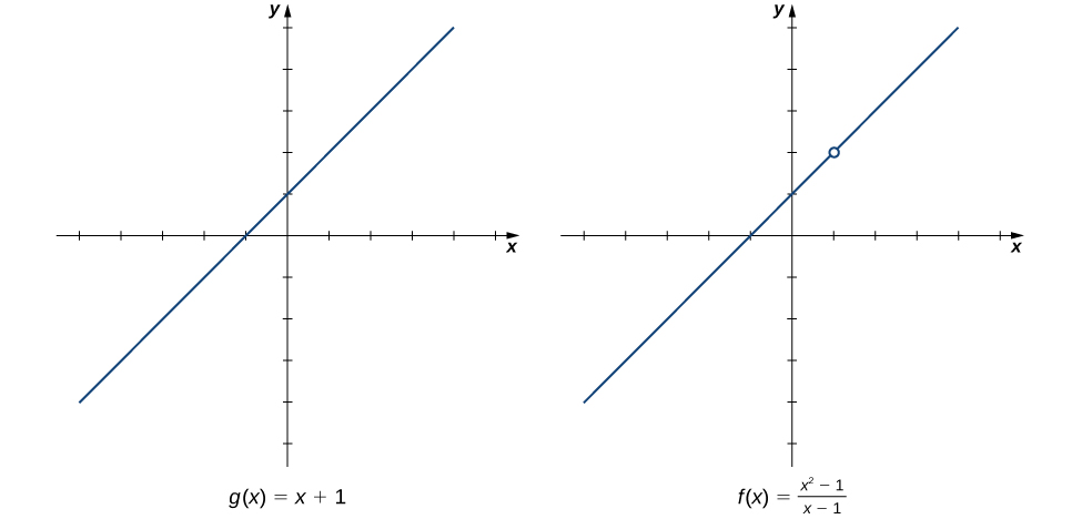
We see that

\[\lim_{x \to 1}\dfrac{x^2−1}{x−1}=\lim_{x \to 1}\dfrac{(x−1)(x+1)}{x−1}=\lim_{x \to 1}\,(x+1)=2.\nonumber \]

The limit has the form \(\displaystyle \lim_{x \to a}f(x)/g(x)\), where \(\displaystyle\lim_{x \to a}f(x)=0\) and \(\displaystyle\lim_{x \to a}g(x)=0\). (In this case, we say that \(f(x)/g(x)\) has the indeterminate form \(0/0\).) When evaluating limits of this type, it is especially important to follow the Mathematical Mantra.

Example \(\PageIndex{4}\): Evaluating a Limit by Factoring and Canceling

Evaluate \(\displaystyle\lim_{x \to 3}\dfrac{x^2−3x}{2x^2−5x−3}\).

Solution

The function \(f(x)=\dfrac{x^2−3x}{2x^2−5x−3}\) is undefined for \(x=3\). In fact, if we substitute 3 into the function we find this limit is indeterminate of the form \(0/0\). This means that we must follow the Mathematical Mantra and perform any arithmetic, algebra, and then trigonometry prior to attempting to apply calculus here.

From our prerequisite algebra, we can see that factoring in both the numerator and denominator is possible.

\[\begin{array}{rclcl}
\displaystyle \lim_{x \to 3}{\frac{x^2−3x}{2x^2−5x−3}} & = & \displaystyle \lim_{x \to 3}{\frac{x(x−3)}{(x−3)(2x+1)}} & & \\
& = & \displaystyle \lim_{x \to 3}{\frac{x\cancel{(x−3)}}{\cancel{(x−3)}(2x+1)}} & & \\
& = & \displaystyle \lim_{x \to 3}{\frac{x}{2x+1}}  & & (\text{Direct Substitution is now applicable}) \\
& \overset{D.S.}{=} & \frac{3}{7}  & &  \\
\end{array} \nonumber \]

Caution: Limits Require... Limits

A very common mistake is to not use limit notation when working with limits. Be aware that limit notation is incredibly important in calculus and must be used up to the moment that you finish evaluating the limit. Example \( \PageIndex{4} \) illustrates proper use of limit notation. The following, however, would be absolutely incorrect:

\(\begin{array}{rcl} \displaystyle \lim_{x \to 3}{\frac{x^2−3x}{2x^2−5x−3}} & = & \displaystyle \lim_{x \to 3}{\frac{x(x−3)}{(x−3)(2x+1)}} \\ & = & \frac{x\cancel{(x−3)}}{\cancel{(x−3)}(2x+1)} \\ & = & \frac{x}{2x+1}  \\ & \overset{D.S.}{=} & \frac{3}{7} \\ \end{array} \)

Exercise \(\PageIndex{4}\)

Evaluate \(\displaystyle \lim_{x \to −3}\dfrac{x^2+4x+3}{x^2−9}\).

Hint

Follow the Mathematical Mantra.

Answer

\(\dfrac{1}{3}\)

Example \(\PageIndex{5}\): Evaluating a Limit by Multiplying by a Conjugate

Suppose we are allowed to assume \( \displaystyle \lim_{t \to 0}{\cosh{(t)} = 1} \) (we normally cannot make any assumptions about the value of a limit that does not involve either polynomial or rational functions; however, we will allow ourselves this assumption for this specific example - and only this once). Evaluate \( \displaystyle \lim_{t \to 0}{\frac{\sqrt{\cosh{(t)} + 3} − 2}{\cosh{(t)} - 1}}\).

Solution

As \(t\) approaches \(0\), both the numerator and denominator of \(f(x)=\frac{\sqrt{\cosh{(t)} + 3} − 2}{\cosh{(t)} - 1}\) approach \(0\). Therefore, this limit is indeterminate of the form \(0/0\). This means that we must follow the Mathematical Mantra and perform any arithmetic, algebra, and then trigonometry (generally, in that order) prior to attempting to apply calculus here.

The numerator, having two terms where one involves a square root, is enticing. Let's try multiplying both numerator and denominator by the conjugate of the numerator.

\[\begin{array}{rclr}
\displaystyle \lim_{t \to 0}{\dfrac{\sqrt{\cosh{(t)} + 3} − 2}{\cosh{(t)} - 1}} & = & \displaystyle \lim_{t \to 0}{\left(\dfrac{\sqrt{\cosh{(t)} + 3} − 2}{\cosh{(t)} - 1} \cdot \dfrac{\sqrt{\cosh{(t)} + 3} + 2}{\sqrt{\cosh{(t)} + 3} + 2}\right)} & \\
& = & \displaystyle \lim_{t \to 0}{\left(\dfrac{\cosh{(t)} + 3 - 4}{\left( \cosh{(t)} - 1 \right) \left( \sqrt{\cosh{(t)} + 3} + 2\right)}\right)} & (\text{Algebra: distribution* (see Note below)}) \\
& = & \displaystyle \lim_{t \to 0}{\left(\dfrac{\cosh{(t)} - 1}{\left( \cosh{(t)} - 1 \right) \left( \sqrt{\cosh{(t)} + 3} + 2\right)}\right)}  & \\
& = & \displaystyle \lim_{t \to 0}{\left(\dfrac{\cancel{(\cosh{(t)} - 1)}}{\cancel{\left( \cosh{(t)} - 1 \right)} \left( \sqrt{\cosh{(t)} + 3} + 2\right)}\right)}  & \\
& = & \displaystyle \lim_{t \to 0}{\left(\dfrac{1}{\sqrt{\cosh{(t)} + 3} + 2}\right)}  & \\
& = & \dfrac{\displaystyle \lim_{t \to 0}{1}}{\displaystyle \lim_{t \to 0}{\left(\sqrt{\cosh{(t)} + 3} + 2\right)}}  & \left( \text{Calculus: Quotient Law for Limits} \right)\\
& = & \dfrac{1}{\displaystyle \lim_{t \to 0}{\sqrt{\cosh{(t)} + 3}} + \lim_{t \to 0}{2}}  & \left( \text{Calculus: Sum Law for Limits and Corollary }\PageIndex{1} \right) \\
& = & \dfrac{1}{\sqrt{\displaystyle \lim_{t \to 0}{\left(\cosh{(t)} + 3\right)}} + 2}  & \left( \text{Calculus: Root Law for Limits and Corollary }\PageIndex{1} \right) \\
& = & \dfrac{1}{\sqrt{\displaystyle \lim_{t \to 0}{\cosh{(t)}} + \displaystyle \lim_{t \to 0}{3}} + 2}  & \left( \text{Calculus: Sum Law for Limits} \right) \\
& = & \dfrac{1}{\sqrt{1 + 3} + 2}  & \left( \text{Calculus: Corollary }\PageIndex{1} \text{ and the given limit} \right) \\
& = & \dfrac{1}{4}  & \\
\end{array} \nonumber \]

Note: Conjugate Multiplication and Distribution

When multiplying the numerator and denominator of an expression by a conjugate (of either the numerator or the denominator), it is advisable to only perform distribution on the conjugate factors.

For example, consider the following two limits

\[ \lim_{x \to -10}{\frac{\sqrt{110 + x} - 10}{x + 10}} \qquad \text{and} \qquad \lim_{\theta \to 0}{\frac{\sin^3{(\theta)}}{1 - \cos{(\theta)}}}  \nonumber \]

Both are indeterminate of the form \(0/0\). Multiplying the numerator and denominator of the first limit by \(\sqrt{110 + x} + 10\) and the numerator and denominator of the second by \(1 + \cos{(\theta)}\), we get

\[ \lim_{x \to -10}{\left( \frac{\sqrt{110 + x} - 10}{x + 10} \cdot \frac{\sqrt{110 + x} + 10}{\sqrt{110 + x} + 10} \right)} \qquad \text{and} \qquad \lim_{\theta \to 0}{\left(\frac{\sin^3{(\theta)}}{1 - \cos{(\theta)}} \cdot \frac{1 + \cos{(\theta)}}{1 + \cos{(\theta)}}\right)}  \nonumber \]

By distributing the conjugate factors and leaving the non-conjugate factors as an undistributed product, we get

\[ \lim_{x \to -10}{\left( \frac{110 + x - 100}{\left(x + 10\right) \left(\sqrt{110 + x} + 10\right)} \right)} \qquad \text{and} \qquad \lim_{\theta \to 0}{\left(\frac{\sin^3{(\theta)} \left( 1 + \cos{(\theta)} \right)}{1 - \cos^2{(\theta)}} \right)}  \nonumber \]

Simplifying...

\[ \lim_{x \to -10}{\left( \frac{10 + x}{\left(x + 10\right) \left(\sqrt{110 + x} + 10\right)} \right)} \qquad \text{and} \qquad \lim_{\theta \to 0}{\left(\frac{\sin^3{(\theta)} \left( 1 + \cos{(\theta)} \right)}{\sin^2{(\theta)}} \right)}  \nonumber \]

... something beautiful occurs!

\[ \lim_{x \to -10}{\left( \frac{\cancel{(10 + x)}}{\cancel{\left(x + 10\right)} \left(\sqrt{110 + x} + 10\right)} \right)} \overset{D.S.}{=} \frac{1}{20} \qquad \text{and} \qquad \lim_{\theta \to 0}{\left( \sin{(\theta)} \left( 1 + \cos{(\theta)} \right) \right)} \overset{D.S.}{=} 0 \nonumber \]

(Note: I did a little bit of "hand-waving" on the Direct Substitution for the trigonometric expression. Technically, we have not learned the Direct Substitution Property for trigonometric functions, but the point of the example here was to showcase when to distribute conjugates and when not to.)

Exercise \(\PageIndex{5}\)

Evaluate \( \displaystyle \lim_{x \to 5}\dfrac{\sqrt{x−1}−2}{x−5}\).

Hint

Follow the Mathematical Mantra.

Answer

\(\dfrac{1}{4}\)

Example \(\PageIndex{6}\): Evaluating a Limit by Simplifying a Complex Fraction

Evaluate \( \displaystyle \lim_{x \to 1}\dfrac{\dfrac{1}{x+1}−\dfrac{1}{2}}{x−1}\).

Solution

As \(x \to 1\), the function \(f(x)=\dfrac{\dfrac{1}{x+1}−\dfrac{1}{2}}{x−1}\) approaches \(0/0\). This means that we must follow the Mathematical Mantra and perform any arithmetic, algebra, and then trigonometry (generally, in this order) prior to attempting to apply calculus.

From our prerequisite algebra, we know that any compound fraction like this should be simplified.

\[\begin{array}{rclcl}
\displaystyle \lim_{x \to 1}{\frac{\frac{1}{x+1}−\frac{1}{2}}{x−1}} & = & \displaystyle \lim_{x \to 1}{\frac{2−(x + 1)}{2(x−1)(x+1)}} & & \\
& = & \displaystyle \lim_{x \to 1}{\frac{1 − x}{2(x−1)(x+1)}} & & \\
& = & \displaystyle \lim_{x \to 1}{\frac{-(x - 1)}{2(x−1)(x+1)}}  & & \\
& = & \displaystyle \lim_{x \to 1}{\frac{-\cancel{(x - 1)}}{2\cancel{(x−1)}(x+1)}}  & & \\
& = & \displaystyle \lim_{x \to 1}{\frac{-1}{2(x+1)}}  & & (\text{Direct Substitution is now applicable}) \\
& \overset{D.S.}{=} & -\frac{1}{4}  & &  \\
\end{array} \nonumber \]

Exercise \(\PageIndex{6}\)

Evaluate \( \displaystyle \lim_{x \to −3}\dfrac{\dfrac{1}{x+2}+1}{x+3}\).

Hint

Follow the Mathematical Mantra.

Answer

−1

Example \(\PageIndex{7}\): Evaluating a Limit Involving Absolute Values

Evaluate \( \displaystyle \lim_{x \to (-5/3)^-}{ \dfrac{|3x + 5|}{6x^2 + 7x - 5} }\).

Solution

As \(x \to (-5/3)^-\), both numerator and denominator of the limit tend to \(0\). Therefore, this limit is indeterminate of the form \(\dfrac{0}{0}\). Following the Mathematical Mantra, we clean things up first by performing some algebra.

Our prerequisite factoring skills allow us to factor the denominator to the following:

\[ 6x^2 + 7x - 5 = (3x + 5)(2x - 1). \nonumber \]

Therefore, 

\[ \displaystyle \lim_{x \to (-5/3)^-}{ \dfrac{|3x + 5|}{6x^2 + 7x - 5} } = \displaystyle \lim_{x \to (-5/3)^-}{ \dfrac{|3x + 5|}{(3x + 5)(2x - 1)} }. \nonumber \]

We know, from our prerequisite algebra, that \(|3x + 5|\) is not the same as \(3x + 5\), so we must use the definition of the absolute value to rewrite \(|3x + 5|\).

\[ |3x + 5| = \begin{cases}
3x + 5 & \text{, if }3x + 5 \geq 0  & \implies x \geq -\dfrac{5}{3} \\
-(3x + 5) & \text{, if }3x + 5 \lt 0  & \implies x \lt -\dfrac{5}{3} \\
\end{cases} \nonumber \]

Since \(x\) is approaching \(-5/3\) from the left, \(x \lt -5/3\). Therefore, \(|3x + 5| = -(3x + 5)\). Hence,

\[ \begin{array}{rclr}
\displaystyle \lim_{x \to (-5/3)^-}{ \dfrac{|3x + 5|}{6x^2 + 7x - 5} } & = & \displaystyle \lim_{x \to (-5/3)^-}{ \dfrac{|3x + 5|}{(3x + 5)(2x - 1)} } & \\
 & = & \displaystyle \lim_{x \to (-5/3)^-}{ \dfrac{-(3x + 5)}{(3x + 5)(2x - 1)} } & (\text{Algebra: definition of the absolute value}) \\
 & = & \displaystyle \lim_{x \to (-5/3)^-}{ \dfrac{-\cancel{(3x + 5)}}{\cancel{(3x + 5)}(2x - 1)} } & \\
 & = & \displaystyle \lim_{x \to (-5/3)^-}{ \dfrac{-1}{2x - 1} } & (\text{Direct Substitution is now applicable}) \\
 & \overset{\text{D.S.}}{=} & \dfrac{-1}{2(-5/3) - 1} & \\
 & = & \dfrac{3}{13} & \\
\end{array} \nonumber \]

Critical Mistake!

Example \( \PageIndex{7} \) should remind you of the fact that \( |f(x)| \) is not necessarily equivalent to \(f(x)\). This is a critical prerequisite skill for calculus and it bears repeating here:

\[ |f(x)| = \begin{cases}
f(x) & \text{, if }f(x) \geq 0 \\
-f(x) & \text{, if }f(x) \lt 0 \\
\end{cases} \nonumber \]

Knowing the piecewise definition of the absolute value function, and using it to manipulate expressions involving absolute values, is a key fundamental component to your success in calculus. Theoretically, lacking this single prerequisite skill will not prevent you from succeeding in calculus; however, in practice, a student who cannot master the understanding of this concept rarely (if ever) passes a calculus course.

Example \(\PageIndex{8}\) does not fall neatly into any of the patterns established in the previous examples. However, with a little creativity, we can still use these same techniques.

Example \(\PageIndex{8}\): Evaluating a Limit When the Limit Laws Do Not Apply

Evaluate \( \displaystyle \lim_{x \to 0}\left(\dfrac{1}{x}+\dfrac{5}{x(x−5)}\right)\).

Solution

Both \(1/x\) and \(5/x(x−5)\) fail to have a limit at zero. Since neither of the two functions has a limit at zero, we cannot apply the Sum Law for limits; we must use a different strategy. In this case, we find the limit by performing addition and then applying one of our previous strategies. Observe that

\[\dfrac{1}{x}+\dfrac{5}{x(x−5)}=\dfrac{x−5+5}{x(x−5)}=\dfrac{x}{x(x−5)}.\nonumber \]

Thus,

\[\lim_{x \to 0}\left(\dfrac{1}{x}+\dfrac{5}{x(x−5)}\right)=\lim_{x \to 0}\dfrac{x}{x(x−5)}=\lim_{x \to 0}\dfrac{1}{x−5}=−\dfrac{1}{5}.\nonumber \]

Exercise \(\PageIndex{8}\)

Evaluate \( \displaystyle \lim_{x \to 3}\left(\dfrac{1}{x−3}−\dfrac{4}{x^2−2x−3}\right)\).

Hint

Use the same technique as Example \(\PageIndex{8}\). Don’t forget to factor \(x^2−2x−3\) before getting a common denominator.

Answer

\(\dfrac{1}{4}\)

Let’s now revisit one-sided limits. Simple modifications in the Limit Laws allow us to apply them to one-sided limits. For example, to apply the Limit Laws to a limit of the form \(\displaystyle \lim_{x \to a^−}h(x)\), we require the function \(h(x)\) to be defined over an open interval of the form \((b,a)\); for a limit of the form \(\displaystyle \lim_{x \to a^+}h(x)\), we require the function \(h(x)\) to be defined over an open interval of the form \((a,c)\). Example \(\PageIndex{9A}\) illustrates this point.

Example \(\PageIndex{9A}\): Evaluating a One-Sided Limit Using the Limit Laws

Evaluate each of the following limits, if possible.

1. \(\displaystyle \lim_{x \to 3^−}\sqrt{x−3}\)
2. \( \displaystyle \lim_{x \to 3^+}\sqrt{x−3}\)

Solution

Figure \(\PageIndex{2}\) illustrates the function \(f(x)=\sqrt{x−3}\) and aids in our understanding of these limits.

Figure \(\PageIndex{2}\): The graph shows the function \(f(x)=\sqrt{x−3}\).

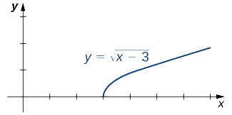
a. The function \(f(x)=\sqrt{x−3}\) is defined over the interval \([3,+\infty)\). Since this function is not defined to the left of 3, we cannot apply the Limit Laws to compute \(\displaystyle\lim_{x \to 3^−}\sqrt{x−3}\). In fact, since \(f(x)=\sqrt{x−3}\) is undefined to the left of 3, \(\displaystyle\lim_{x \to 3^−}\sqrt{x−3}\) does not exist.

b. Since \(f(x)=\sqrt{x−3}\) is defined to the right of 3, the Limit Laws do apply to \(\displaystyle\lim_{x \to 3^+}\sqrt{x−3}\). By applying these Limit Laws we obtain \(\displaystyle\lim_{x \to 3^+}\sqrt{x−3}=0\).

In Example \(\PageIndex{9B}\) we look at one-sided limits of a piecewise-defined function and use these limits to draw a conclusion about a two-sided limit of the same function.

Example \(\PageIndex{9B}\): Evaluating a Two-Sided Limit Using the Limit Laws

For \(f(x)=\begin{cases}4x−3, & \mathrm{if} \; x<2 \\ (x−3)^2, & \mathrm{if} \; x \geq 2\end{cases}\), evaluate each of the following limits:

1. \(\displaystyle \lim_{x \to 2^−}f(x)\)
2. \(\displaystyle \lim_{x \to 2^+}f(x)\)
3. \(\displaystyle \lim_{x \to 2}f(x)\)

Solution

Figure \(\PageIndex{3}\) illustrates the function \(f(x)\) and aids in our understanding of these limits.

Figure \(\PageIndex{3}\): This graph shows a function \(f(x)\).

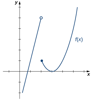
a. Since \(f(x)=4x−3\) for all \(x\) in \((−\infty,2)\), replace \(f(x)\) in the limit with \(4x−3\) and apply the Limit Laws:

\[\lim_{x \to 2^−}f(x)=\lim_{x \to 2^−}(4x−3)=5\nonumber \]

b. Since \(f(x)=(x−3)^2\)for all \(x\) in \((2,+\infty)\), replace \(f(x)\) in the limit with \((x−3)^2\) and apply the Limit Laws:

\[\lim_{x \to 2^+}f(x)=\lim_{x \to 2^−}(x−3)^2=1. \nonumber \]

c. Since \(\displaystyle \lim_{x \to 2^−}f(x)=5\) and \(\displaystyle \lim_{x \to 2^+}f(x)=1\), we conclude that \(\displaystyle \lim_{x \to 2}f(x)\) does not exist.

Exercise \(\PageIndex{9}\)

Graph \(f(x)=\begin{cases}−x−2, & \mathrm{if} \; x<−1\\ 2, & \mathrm{if} \; x=−1 \\ x^3, & \mathrm{if} \; x>−1\end{cases}\) and evaluate \(\displaystyle \lim_{x \to −1^−}f(x)\).

Hint

Use the method in Example \(\PageIndex{8B}\) to evaluate the limit.

Answer

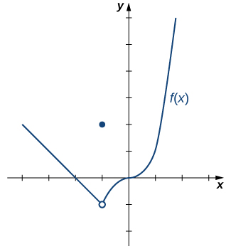
\[\lim_{x \to −1^−}f(x)=−1\nonumber \]

---

Where the Limit Laws Break

As stated in earlier, the Limit Laws can only be applied when the component limits are finite. A very common mistake made early on in a calculus course is to think that you can apply the Limit Laws to any given limit - again, this is not true.

Example \(\PageIndex{10}\): Breaking the (Limit) Laws

Evaluate each of the following limits.

1. \( \displaystyle \lim_{x \to 3^+}{\left( (x-3) \cdot \frac{1}{x-3} \right)} \)
2. \( \displaystyle \lim_{x \to 3^-}{\left( (x-3)^2 \cdot \frac{1}{x-3} \right)} \)
3. \( \displaystyle \lim_{x \to 3^+}{\left( (x-3) \cdot \frac{1}{(x-3)^3} \right)} \)

Solution

1. If we were to try to apply the Product Law for Limits, we would arrive at
   \[\displaystyle \lim_{x \to 3^+}{(x-3)} \cdot \displaystyle \lim_{x \to 3^+}{\frac{1}{x-3}} = 0 \cdot \infty = 0 \text{ or is it } \infty? \nonumber\]
   This is wrong on several levels.
   First, what is the product of something approaching \(0\) and something approaching \(\infty\)? This is a key difference between algebra and calculus. In algebra, you are consistently dealing with finite values and, as such, the rules of arithmetic apply neatly. In calculus, you are dealing with levels of infinity (and the infinitesimal). These concepts do not obey the traditional rules of arithmetic.
   The second issue is that we are breaking the Limit Laws! Remember, you can only use the Limit Laws if the component limits exist and are finite.
   So, how would you deal with the given limit? Using the Mathematical Mantra, we perform some very simple algebra.
   \[\displaystyle \lim_{x \to 3^+}{\left( (x-3) \cdot \frac{1}{x-3} \right)} = \displaystyle \lim_{x \to 3^+}{\left( \cancel{(x-3)} \cdot \frac{1}{\cancel{(x-3)}} \right)} = \displaystyle \lim_{x \to 3^+}{1} = 1 \nonumber\]
2. Trying to apply the Product Law for Limits, we would get
   \[\displaystyle \lim_{x \to 3^-}{(x-3)^2} \cdot \displaystyle \lim_{x \to 3^-}{\frac{1}{x-3}} = 0 \cdot -\infty = 0 \text{ or is it } -\infty? \nonumber\]
   Just like part a, we are improperly trying to apply the Limit Laws in a situation where they are not applicable. That second limit, approaching \(-\infty\), prevents us from using the Limit Laws. Instead, the proper way to evaluate this limit is to use some simple algebra first.
   \[\displaystyle \lim_{x \to 3^-}{\left( (x-3)^2 \cdot \frac{1}{x-3} \right)} = \displaystyle \lim_{x \to 3^-}{(x-3)} = 0 \nonumber\]
3. Again, incorrectly applying the Product Law for Limits, we would get
   \[\displaystyle \lim_{x \to 3^+}{(x-3)} \cdot \displaystyle \lim_{x \to 3^+}{\frac{1}{(x-3)^3}} = 0 \cdot \infty = 0 \text{ or is it } \infty? \nonumber\]
   As in the previous two examples, we are breaking the Limit Laws because one of the component limits is not finite. We should have performed some simple algebra first.
   \[\displaystyle \lim_{x \to 3^+}{\left( (x-3) \cdot \frac{1}{(x-3)^3} \right)} = \displaystyle \lim_{x \to 3^+}{\left( \frac{1}{\cancel{(x-3)^2}} \right)} = \infty \nonumber\]

Pay close attention to Example \(\PageIndex{10}\). It should serve as a warning that anytime you reach an "answer" of the form \(0 \cdot \infty\), you are wrong - period.

---

The Squeeze Theorem

The techniques we have developed thus far work very well for algebraic functions, but we are still unable to evaluate limits of very basic trigonometric functions. The next theorem, called the Squeeze Theorem, proves very useful for establishing basic trigonometric limits. It also helps us evaluate very abstract and theoretical limits for functions that cannot be described using simple functions from our algebra courses. This theorem allows us to calculate limits by “squeezing” a function, with a limit at a point \(a\) that is unknown, between two functions having a common known limit at \(a\). Figure \(\PageIndex{4}\) illustrates this idea.

Figure \(\PageIndex{4}\): The Squeeze Theorem applies when \(f(x) \leq g(x) \leq h(x)\) and \(\displaystyle \lim_{x \to a}f(x)=\lim_{x \to a}h(x)\).

Theorem \(\PageIndex{4}\): Squeeze Theorem

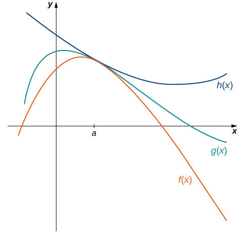
Let \(f(x),g(x)\), and \(h(x)\) be defined for all \(x \neq a\) over an open interval containing \(a\). If

\[f(x) \leq g(x) \leq h(x) \nonumber \]

for all \(x \neq a\) in an open interval containing \(a\) and

\[\lim_{x \to a}f(x)=L=\lim_{x \to a}h(x) \nonumber \]

where \(L\) is a real number, then \(\displaystyle \lim_{x \to a}g(x)=L.\)

Example \(\PageIndex{11}\): Applying the Squeeze Theorem

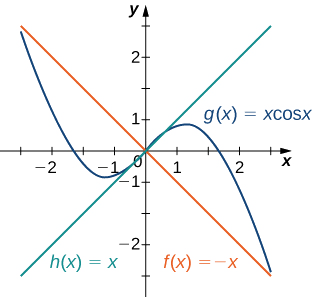
Evaluate \(\displaystyle \lim_{x \to 0}{\left(x\cos{(x)}\right)}\).

Solution

If we were to try to evaluate this limit using the Limit Laws, we would arrive at

\[\displaystyle \lim_{x \to 0}{\left(x\cos{(x)}\right)} = \displaystyle \lim_{x \to 0}{(x)} \cdot \displaystyle \lim_{x \to 0}{\cos{(x)}} = 0 \cdot \text{... ummm... what is this?} \nonumber \]

I get it, you are going to say, "But, I know that \(\cos{(x)}\) approaches \(1\) as \(x\) approaches \(0\)!" However, our theory up to this point only includes algebraic functions (specifically, polynomial and rational functions). Therefore, our "intuition" of what this limit will be is not allowed.

We have the limit of the product of two functions. We know the limit of one of those functions; however, if we don't know the limit of the other function, or if we know the limit of the other function does not exist, the Squeeze Theorem can be very helpful if you can bound the function with the unknown or undefined limit.

In this case, we don't (officially) know the limit of the cosine as \(x\) is approaching \(1\). So, we build a bound for this function.

\[ -1 \le \cos{(x)} \le 1 \nonumber \]

We now rebuild the original limit by multiplying all three "sides" of this inequality by \(x\). Before we do so, it is important to note two things: \(x \neq 0\) and we don't know the sign of \(x\). The first statement is just peripherally important so we know that we are not getting something trivial like \(0 \le 0 \le 0\). The second statement is just for completeness. If \(x \gt 0\), then we would get

\[ -x \le x \cos{(x)} \le x \nonumber \]

If \(x \lt 0\), then the inequality signs switch direction to

\[ -x \ge x \cos{(x)} \ge x \nonumber \]

In either case, since \( \displaystyle \lim_{x \to 0}{(-x)} = 0 = \displaystyle \lim_{x \to 0}{(x)} \), from the Squeeze Theorem, we obtain \( \displaystyle \lim_{x \to 0}{(x \cos{(x)})} = 0 \). The graphs of \(f(x)=−x,\;g(x)=x\cos x\), and \(h(x)=x\) are shown in Figure \(\PageIndex{5}\).

Figure \(\PageIndex{5}\): The graphs of \(f(x),\,g(x)\), and \(h(x)\) are shown around the point \(x=0\).

Exercise \(\PageIndex{11}\)

Use the Squeeze Theorem to evaluate \(\displaystyle \lim_{x \to 0}x^2 \sin\dfrac{1}{x}\).

Hint

Use the fact that \(−x^2 \leq x^2\sin (1/x) \leq x^2\) to help you find two functions such that \(x^2\sin (1/x)\) is squeezed between them.

Answer

0

---

Limits Involving the Sine and Cosine

We now use the Squeeze Theorem to tackle several very important limits presented as a theorem here. Although this discussion is somewhat lengthy, these limits prove invaluable for the development of the material in both the next section and the next chapter.

Theorem \(\PageIndex{5}\)

\[ \displaystyle \lim_{\theta \to 0}{\left(\sin{(\theta)}\right)} = 0 \nonumber \]

and

\[ \displaystyle \lim_{\theta \to 0}{\left(\cos{(\theta)}\right)} = 1 \nonumber\]

Proof

The first of these limits is \( \displaystyle \lim_{\theta \to 0}{\left( \sin{(\theta)} \right)} \). Consider the unit circle shown in Figure \(\PageIndex{6}\). In the figure, we see that \(\sin{(\theta)}\) is the \(y\)-coordinate on the unit circle and it corresponds to the line segment shown in blue. The radian measure of angle \(\theta\) is the length of the arc it subtends on the unit circle. Therefore, we see that for \(0 \lt \theta \lt \dfrac{\pi}{2},\) we have \(0 \lt \sin{(\theta)} \lt \theta.\)

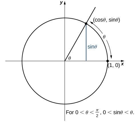
Figure \(\PageIndex{6}\): The sine function is shown as a line on the unit circle.

Because \(\displaystyle \lim_{\theta \to 0^+} 0 = 0\) and \(\displaystyle \lim_{\theta \to 0^+} \theta =0\), by using the Squeeze Theorem we conclude that

\[\lim_{\theta \to 0^+}{\left( \sin{(\theta)} \right)} = 0.\nonumber \]

To see that \(\displaystyle \lim_{\theta \to 0^−}{\left( \sin{(\theta)} \right) } = 0\) as well, observe that for \(−\dfrac{\pi}{2} \lt \theta \lt 0, 0 \lt −\theta \lt \dfrac{\pi}{2}\) and hence, \(0 \lt \sin{(−\theta)} \lt −\theta\). Consequently, \(0 \lt −\sin{(\theta)} \lt −\theta\). It follows that \(0 \gt \sin{(\theta)} \gt \theta\). An application of the Squeeze Theorem produces the desired limit. Thus, since \(\displaystyle \lim_{\theta \to 0^+}{\sin{(\theta)}} = 0\) and \(\displaystyle \lim_{\theta \to 0^−}{\sin{(\theta)}} = 0\),

\[\lim_{\theta \to 0}{\sin{(\theta)}} = 0\nonumber \]

Next, using the identity \(\cos{(\theta)}=\sqrt{1−\sin^2{(\theta)}}\) for \(−\dfrac{\pi}{2} \lt \theta \lt \dfrac{\pi}{2}\), we see that

\[\lim_{\theta \to 0}{(\cos{(\theta)})} = \lim_{\theta \to 0}{\sqrt{1−\sin^2{(\theta)}}} = 1.\nonumber \]

We now take a look at two limits that play important roles in later chapters.

Theorem \(\PageIndex{6}\)

\[ \displaystyle \lim_{\theta \to 0}{\frac{\sin{\theta}}{\theta} } = 1 \nonumber \]

and

\[ \displaystyle \lim_{\theta \to 0}{\frac{1 - \cos{\theta}}{\theta} } = 0 \nonumber \]

Proof

To prove the first of these limits, we use the unit circle in Figure \(\PageIndex{7}\). Notice that this figure adds one additional triangle to Figure \(\PageIndex{6}\) from the proof of Theorem \(\PageIndex{5}\). We see that the length of the side opposite angle \(\theta\) in this new triangle is \(\tan{(\theta)}\). Thus, we see that for \(0 \lt \theta \lt \dfrac{\pi}{2}\), we have \(\sin{(\theta)} \lt \theta \lt \tan{(\theta)}\).

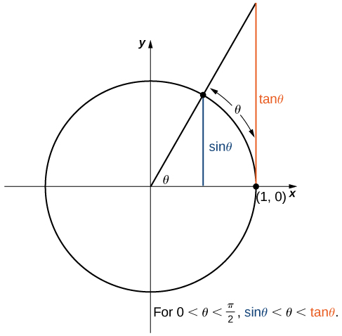
Figure \(\PageIndex{7}\): The sine and tangent functions are shown as lines on the unit circle.

By dividing by \(\sin{(\theta)}\) in all parts of the inequality, we obtain

\[1 \lt \dfrac{\theta}{\sin{(\theta)}} \lt \dfrac{1}{\cos{(\theta)}}.\nonumber \]

Equivalently, we have

\[1 \gt \dfrac{\sin{(\theta)}}{\theta} \gt \cos{(\theta)}.\nonumber \]

Since \(\displaystyle \lim_{\theta \to 0^+}1 = 1 = \lim_{\theta \to 0^+}\cos{(\theta)}\), we conclude that \(\displaystyle \lim_{\theta \to 0^+}\dfrac{\sin{(\theta)}}{\theta} = 1\), by the Squeeze Theorem. By applying a manipulation similar to that used in demonstrating that \(\displaystyle \lim_{\theta \to 0^-}{(\sin{(\theta)})} = 0\), we can show that \(\displaystyle \lim_{\theta \to 0^−}\dfrac{\sin{(\theta)}}{\theta} = 1\). Thus,

\[\lim_{\theta \to 0}\dfrac{\sin{(\theta)}}{\theta}=1. \nonumber \]

In Example \(\PageIndex{12}\), we use this limit to establish \(\displaystyle \lim_{\theta \to 0}\dfrac{1−\cos{(\theta)}}{\theta}=0\). This limit also proves useful in later chapters.

Example \(\PageIndex{12}\): Evaluating an Important Trigonometric Limit

Evaluate \(\displaystyle \lim_{ \theta \to 0 }\dfrac{1−\cos \theta }{ \theta }\).

Solution

In the first step, we multiply by the conjugate so that we can use a trigonometric identity to convert the cosine in the numerator to a sine:

\[\begin{align*} \lim_{ \theta \to 0}\dfrac{1−\cos \theta }{ \theta } &=\displaystyle \lim_{ \theta \to 0}\dfrac{1−\cos \theta }{ \theta } \cdot \dfrac{1+\cos \theta }{1+\cos \theta }\\[4pt]
&= \lim_{ \theta \to 0}\dfrac{1−\cos^2 \theta }{ \theta (1+\cos \theta )}\\[4pt]
&= \lim_{ \theta \to 0}\dfrac{\sin^2 \theta }{ \theta (1+\cos \theta )}\\[4pt]
&= \lim_{ \theta \to 0}\dfrac{\sin \theta }{ \theta } \cdot \dfrac{\sin \theta }{1+\cos \theta }\\[4pt]
&= \left(\lim_{ \theta \to 0}\dfrac{\sin \theta }{ \theta } \right)\cdot\left( \lim_{ \theta \to 0} \dfrac{\sin \theta }{1+\cos \theta }\right) \\[4pt]
&= 1 \cdot \dfrac{0}{2}=0. \end{align*}\]

Therefore,

\[\lim_{ \theta \to 0}\dfrac{1−\cos \theta }{ \theta }=0. \nonumber \]

Example \(\PageIndex{13}\): Evaluating Finite Limits of Trigonometric Functions at Finite Points

Evaluate the following limit.

\[ \displaystyle \lim_{\theta \to 0}{\frac{7\theta}{\sin{(5\theta)}}} \nonumber \]

Solution

\[ \begin{array}{rclr}
 \displaystyle \lim_{\theta \to 0}{\dfrac{7\theta}{\sin{(5\theta)}}} & = & \displaystyle \lim_{\theta \to 0}{\dfrac{\frac{7}{5}}{\frac{\sin{(5\theta)}}{5 \theta}}} & \\
 & = & \dfrac{\displaystyle \lim_{\theta \to 0}{\frac{7}{5}}}{\displaystyle \lim_{\theta \to 0}{\frac{\sin{(5\theta)}}{5 \theta}}} & (\text{Calculus: Limit Law}) \\
 & = & \dfrac{\frac{7}{5}}{\displaystyle \lim_{\theta \to 0}{\frac{\sin{(5\theta)}}{5 \theta}}} & (\text{Calculus: Limit Law}) \\
 & = & \dfrac{7}{5} \cdot \dfrac{1}{\displaystyle \lim_{x \to 0}{\frac{\sin{(x)}}{x}}} & (\text{Calculus: Let }x = 5\theta\text{. Then }x \to 0\text{ as }\theta \to 0) \\ 
 & \overset{\text{D.S.}}{=} & \dfrac{7}{5}\cdot \dfrac{1}{1} & \\
 & = & \dfrac{7}{5} & \\
\end{array}
\nonumber \]

Exercise \(\PageIndex{13}\)

Evaluate \(\displaystyle \lim_{ \theta \to 0}\dfrac{1−\cos \theta }{\sin \theta }\).

Hint

Multiply numerator and denominator by \(1+\cos \theta \).

Answer

0

Deriving the Formula for the Area of a Circle

Some of the geometric formulas we take for granted today were first derived by methods that anticipate some of the methods of calculus. The Greek mathematician Archimedes (ca. 287−212; BCE) was particularly inventive, using polygons inscribed within circles to approximate the area of the circle as the number of sides of the polygon increased. He never came up with the idea of a limit, but we can use this idea to see what his geometric constructions could have predicted about the limit.

We can estimate the area of a circle by computing the area of an inscribed regular polygon. Think of the regular polygon as being made up of \(n\) triangles. By taking the limit as the vertex angle of these triangles goes to zero, you can obtain the area of the circle. To see this, carry out the following steps:

1.Express the height \(h\) and the base \(b\) of the isosceles triangle in Figure \(\PageIndex{8}\) in terms of \( \theta \) and \(r\).

Figure \(\PageIndex{8}\)

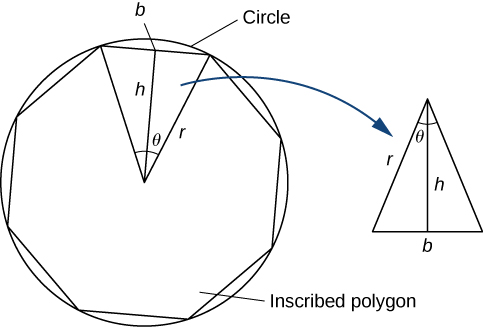
2. Using the expressions that you obtained in step 1, express the area of the isosceles triangle in terms of \( \theta \) and \(r\).

(Substitute \(\frac{1}{2}\sin \theta \) for \(\sin\left(\frac{ \theta }{2}\right)\cos\left(\frac{ \theta }{2}\right)\) in your expression.)

3. If an \(n\)-sided regular polygon is inscribed in a circle of radius \(r\), find a relationship between \( \theta \) and \(n\). Solve this for \(n\). Keep in mind there are \(2 \pi \) radians in a circle. (Use radians, not degrees.)

4. Find an expression for the area of the \(n\)-sided polygon in terms of \(r\) and \( \theta \).

5. To find a formula for the area of the circle, find the limit of the expression in step 4 as \( \theta \) goes to zero. (Hint: \(\displaystyle \lim_{ \theta \to 0}\dfrac{\sin \theta }{ \theta }=1)\).

The technique of estimating areas of regions by using polygons is revisited in Introduction to Integration.

---

Key Concepts

• The Limit Laws allow us to evaluate finite limits of functions without having to go through step-by-step processes each time.
• For polynomials and rational functions, \[\lim_{x \to a}f(x)=f(a). \nonumber \]
• You can evaluate the limit of a function by factoring and canceling, by multiplying by a conjugate, or by simplifying a complex fraction.
• The Squeeze Theorem allows you to find the limit of a function if the function is always greater than one function and less than another function with limits that are known.

---

Key Equations

• Basic Limit Results

\[\lim_{x \to a}x=a \quad \quad \lim_{x \to a}c=c \nonumber \]

• Important Limits

\[ \lim_{ \theta \to 0}\sin \theta =0 \nonumber \]

\[ \lim_{ \theta \to 0}\cos \theta =1 \nonumber \]

\[ \lim_{ \theta \to 0}\dfrac{\sin \theta }{ \theta }=1 \nonumber \]

\[ \lim_{ \theta \to 0}\dfrac{1−\cos \theta }{ \theta }=0 \nonumber \]

---

Common Mistakes

• Prerequisite Mistakes
  • Bad factoring
  • Not understanding conjugate multiplication
  • Low proficiency with negative exponents
  • Not knowing the graphs of prerequisite algebraic and transcendental functions
• Using the Limit Laws on functions whose limits are not finite
• Using a table to estimate the value of a limit
• Not properly bounding a function whose limit is unknown or does not exist when using the Squeeze Theorem.
• Not understanding that when the denominator within a limit is approaching zero, it doesn't equal zero. Division by zero does not occur in calculus; however, division by smaller and smaller values approaching zero occurs very often. Analyzing the ramification of those denominators approaching zero is important in calculus.

---

Glossary

Constant Multiple Law for limits

the limit law \[\lim_{x \to a}cf(x)=c \cdot \lim_{x \to a}f(x)=cL \nonumber \]

difference law for limits

the limit law \[\lim_{x \to a}(f(x)−g(x))=\lim_{x \to a}f(x)−\lim_{x \to a}g(x)=L−M\nonumber \]

Limit Laws

the individual properties of limits; for each of the individual laws, let \(f(x)\) and \(g(x)\) be defined for all \(x \neq a\) over some open interval containing a; assume that L and M are real numbers so that \(\lim_{x \to a}f(x)=L\) and \(\lim_{x \to a}g(x)=M\); let c be a constant

Power Law for limits

the limit law \[\lim_{x \to a}(f(x))^n=(\lim_{x \to a}f(x))^n=L^n\nonumber \]for every positive integer n

product law for limits

the limit law \[\lim_{x \to a}(f(x) \cdot g(x))=\lim_{x \to a}f(x) \cdot \lim_{x \to a}g(x)=L \cdot M\nonumber \]

Quotient Law for limits

the limit law \(\lim_{x \to a}\dfrac{f(x)}{g(x)}=\dfrac{\lim_{x \to a}f(x)}{\lim_{x \to a}g(x)}=\dfrac{L}{M}\) for M \neq 0

root law for limits

the limit law \(\lim_{x \to a}\sqrt[n]{f(x)}=\sqrt[n]{\lim_{x \to a}f(x)}=\sqrt[n]{L}\) for all L if n is odd and for \(L \geq 0\) if n is even

Squeeze Theorem

states that if \(f(x) \leq g(x) \leq h(x)\) for all \(x \neq a\) over an open interval containing a and \(\lim_{x \to a}f(x)=L=\lim_ {x \to a}h(x)\) where L is a real number, then \(\lim_{x \to a}g(x)=L\)

Sum Law for limits

The limit law \(\lim_{x \to a}(f(x)+g(x))=\lim_{x \to a}f(x)+\lim_{x \to a}g(x)=L+M\)