2.4: The Limit Laws - Limits at Infinity

Learning Objectives

• Calculate the limit of a function as \(x\) increases or decreases without bound.
• Define a horizontal asymptote in terms of a finite limit at infinity.
• Evaluate a finite limit at infinity by initially performing algebraic manipulations.
• Conceptually investigate an infinite limit at infinity.
• Describe when the Limit Laws cannot be applied.

In this section, we continue delving into limits by considering limits as \(x\) tends to \(\pm \infty\). These are known collectively as limits at infinity.

---

Finite Limits at Infinity and Horizontal Asymptotes

Recall that \(\displaystyle \lim_{x \to a}f(x)=L\) means \(f(x)\) becomes arbitrarily close to \(L\) as long as \(x\) is sufficiently close to \(a\). We can extend this idea to limits at infinity. For example, consider the function \(f(x)=2+\frac{1}{x}\). As can be seen graphically in Figure \(\PageIndex{1}\) and numerically in Table \(\PageIndex{1}\), as the values of \(x\) get larger, the values of \(f(x)\) approach \(2\). We say the limit as \(x\) approaches \(\infty\) of \(f(x)\) is \(2\) and write \(\displaystyle \lim_{x \to \infty}f(x)=2\). Similarly, for \(x<0\), as the values \(|x|\) get larger, the values of \(f(x)\) approach \(2\). We say the limit as \(x\) approaches \(−\infty\) of \(f(x)\) is \(2\) and write \(\displaystyle \lim_{x \to −\infty}f(x)=2\).

Figure \(\PageIndex{1}\):The function approaches the asymptote \(y=2\) as \(x\) approaches \( \pm \infty\).

Table \(\PageIndex{1}\): Values of a function \(f\) as \(x \to \pm \infty\)

\(x\)	10	100	1,000	10,000
\(2+\frac{1}{x}\)	2.1	2.01	2.001	2.0001
\(x\)	−10	−100	−1000	−10,000
\(2+\frac{1}{x}\)	1.9	1.99	1.999	1.9999

More generally, for any function \(f\), we say the limit as \(x \to \infty\) of \(f(x)\) is \(L\) if \(f(x)\) becomes arbitrarily close to \(L\) as long as \(x\) is sufficiently large. In that case, we write \(\displaystyle \lim_{x \to \infty}f(x)=L\). Similarly, we say the limit as \(x \to −\infty\) of \(f(x)\) is \(L\) if \(f(x)\) becomes arbitrarily close to \(L\) as long as \(x<0\) and \(|x|\) is sufficiently large. In that case, we write \(\displaystyle \lim_{x \to −\infty}f(x)=L\). We now look at the definition of a function having a limit at infinity.

Definition: Finite Limit at Infinity (Informal)

If the values of \(f(x)\) become arbitrarily close to the finite value \(L\) as \(x\) becomes sufficiently large, we say the function \(f\) has a finite limit at infinity and write

\[\lim_{x \to \infty}f(x)=L. \nonumber \]

If the values of \(f(x)\) becomes arbitrarily close to the finite value \(L\) for \(x<0\) as \(|x|\) becomes sufficiently large, we say that the function \(f\) has a finite limit at negative infinity and write

\[\lim_{x \to −\infty}f(x)=L. \nonumber \]

If the values \(f(x)\) are getting arbitrarily close to some finite value \(L\) as \(x \to \infty\) or \(x \to −\infty\), the graph of \(f\) approaches the line \(y=L\). In that case, the line \(y=L\) is a horizontal asymptote of \(f\) (Figure \(\PageIndex{2}\)). For example, for the function \(f(x)=\dfrac{1}{x}\), since \(\displaystyle \lim_{x \to \infty}f(x)=0\), the line \(y=0\) is a horizontal asymptote of \(f(x)=\dfrac{1}{x}\).

Figure \(\PageIndex{2}\): (a) As \(x \to \infty\), the values of \(f\) are getting arbitrarily close to \(L\). The line \(y=L\) is a horizontal asymptote of \(f\). (b) As \(x \to −\infty\), the values of \(f\) are getting arbitrarily close to \(M\). The line \(y=M\) is a horizontal asymptote of \(f\).

Definition: Horizontal Asymptote

If \(\displaystyle \lim_{x \to \infty}f(x)=L\) or \(\displaystyle \lim_{x \to −\infty}f(x)=L\), we say the line \(y=L\) is a horizontal asymptote of \(f\).

As a very important aside, we know from our prerequisite algebra that a function cannot intersect a vertical asymptote; however, a function can cross a horizontal asymptote. In fact, a function may cross a horizontal asymptote an unlimited number of times. For example, the function \(f(x)=\dfrac{\cos x}{x}+1\) shown in Figure \(\PageIndex{3}\) intersects the horizontal asymptote \(y=1\) an infinite number of times as it oscillates around the asymptote with ever-decreasing amplitude.

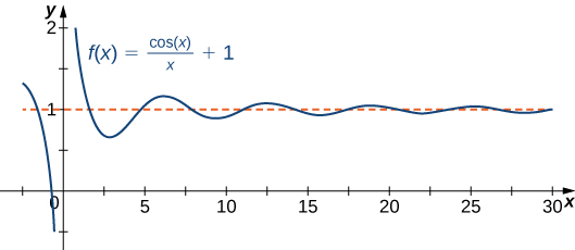
Figure \(\PageIndex{3}\): The graph of \(f(x)=(\cos x)/x+1\) crosses its horizontal asymptote \(y=1\) an infinite number of times.

---

Revisiting the Limit Laws

Now that we have an informal definition of a finite limit at infinity, it's time we begin evaluating some limits without resorting to building tables of values. Before we do, however, we need some theory. The Limit Laws introduced earlier in this chapter still apply as long as the limit values are finite. These are restated here for your convenience.

Theorem \(\PageIndex{1}\): Limit Laws for Limits at Infinity

Let \(f(x)\) and \(g(x)\) be defined for all \(x \gt a\), where \(a\) is a real number. Assume that \(L\) and \(M\) are real numbers such that \(\displaystyle \lim_{x \to \infty}{f(x)} = L\) and \(\displaystyle \lim_{x \to \infty}{g(x)} = M\). Let \(c\) be a constant. Then, each of the following statements holds:

• Sum and Difference Laws for Limits:

\[\displaystyle \lim_{x \to \infty}{(f(x) \pm g(x))} = \lim_{x \to \infty}{f(x)} \pm \lim_{x \to \infty}{g(x)} = L \pm M \nonumber \]

• Constant Multiple Law for Limits:

\[\displaystyle \lim_{x \to \infty}{cf(x)} = c \cdot \lim_{x \to \infty}{f(x)} = c L \nonumber \]

• Product Law for Limits:

\[\displaystyle \lim_{x \to \infty}{(f(x) \cdot g(x))} = \lim_{x \to \infty}{f(x)} \cdot \lim_{x \to \infty}{g(x)} = L \cdot M \nonumber \]

• Quotient Law for Limits:

\[\displaystyle \lim_{x \to \infty}\frac{f(x)}{g(x)} = \frac{\displaystyle \lim_{x \to \infty}f(x)}{\displaystyle \lim_{x \to \infty}g(x)}=\frac{L}{M} \nonumber \]

for \(M \neq 0\).

• Power Law for Limits:

\[\displaystyle \lim_{x \to \infty}\big(f(x)\big)^n = \big(\lim_{x \to \infty}f(x)\big)^n = L^n \nonumber \]

for every positive integer \(n\).

• Root Law for Limits:

\[\displaystyle \lim_{x \to \infty}\sqrt[n]{f(x)} = \sqrt[n]{\lim_{x \to \infty} f(x)}=\sqrt[n]{L} \nonumber \]

for all \(L\) if \(n\) is odd and for \(L \geq 0\) if \(n\) is even.

Each of these Limit Laws can be adjusted for \(x \to -\infty\) as long as \(f(x)\) and \(g(x)\) are defined for all \(x \lt a\), where \(a\) is a real number.

We add to our theory arsenal a small, but powerful lemma.

Lemma \(\PageIndex{1}\)

\[ \displaystyle \lim_{x \to \infty}{x} = \infty, \nonumber \]

\[ \displaystyle \lim_{x \to -\infty}{x} = -\infty, \nonumber \]

and

\[ \displaystyle \lim_{x \to \pm \infty}{\frac{1}{x}} = 0. \nonumber \]

While the results of this lemma are intuitively obvious, we will still prove them once we reach the precise definition of a limit later in this chapter. For now, this lemma allows us to prove the following theorem.

Theorem \(\PageIndex{2}\)

If \(p \gt 0\) is a rational number, then

\[ \displaystyle \lim_{x \to \infty}{\frac{1}{x^p}} = 0. \nonumber \]

If \(p \gt 0 \) is a rational number such that \(x^p\) is defined for all \(x\), then

\[ \displaystyle \lim_{x \to -\infty}{\frac{1}{x^p}} = 0. \nonumber \]

Proof

Let \(p\) be a rational number. The only constraint on using the Limit Laws is that the values of the limits must be finite. Therefore, \(a\) is allowed to be \(\pm \infty\). Thus,
\[ \begin{array}{rclcl} \displaystyle \lim_{x \to \infty}{\frac{1}{x^p}} & = & \displaystyle \lim_{x \to \infty}{\left(\frac{1}{x}\right)^p} & & \\ & = & \left(\displaystyle \lim_{x \to \infty}{\frac{1}{x}} \right)^p & & (\text{a mixture of the Power Law and Root Law for Limits}) \\ & = & 0^p & & (\text{by Lemma }\PageIndex{1}) \\ & = & 0 & & \\ \end{array} \nonumber \]
If we allow \(x \to -\infty\), then additional restrictions on \(p\) must be made. Specifically, since \(p\) is a rational number, it cannot be equivalent to a simplified fraction with an even denominator. Otherwise, the even denominator would imply an even-indexed root of \(x\), and this would result in imaginary numbers. Hence, as long as \(x^p\) is defined,
\[ \displaystyle \lim_{x \to -\infty}{\frac{1}{x^p}} = 0 \nonumber \]
by a similar derivation.

---

Evaluating Finite Limits at Infinity

Example \(\PageIndex{1}\): Computing a Finite Limit at Infinity

Evaluate

\[ \displaystyle \lim_{x \to \infty}{\left(5−\dfrac{2}{x^2}\right)} \nonumber \]

and

\[\displaystyle \lim_{x \to -\infty}{\left(5−\dfrac{2}{x^2}\right)}. \nonumber \]

Determine the horizontal asymptote(s) for this function.

Solution

Using the Limit Laws, we have

\[\lim_{x \to \infty}{\left(5−\frac{2}{x^2}\right)} = \lim_{x \to \infty}5−2\left(\lim_{x \to \infty}{\frac{1}{x}}\right)^2=5−2 \cdot 0=5.\nonumber \]

Similarly, \(\displaystyle \lim_{x \to -\infty}{\left(5−\frac{2}{x^2}\right)}=5\). Therefore, \(f(x)=5-\dfrac{2}{x^2}\) has a horizontal asymptote of \(y=5\) and \(f\) approaches this horizontal asymptote as \(x \to \pm \infty\) as shown in the following graph.

Figure \(\PageIndex{4}\): This function approaches a horizontal asymptote as \(x \to \pm \infty.\)

Exercise \(\PageIndex{1}\)

Evaluate \(\displaystyle \lim_{x \to −\infty}\left(3+\frac{4}{x}\right)\) and \(\displaystyle \lim_{x \to \infty}\left(3+\dfrac{4}{x}\right)\). Determine the horizontal asymptotes of \(f(x)=3+\frac{4}{x},\) if any.

Hint

\(\displaystyle \lim_{x \to \pm \infty}\frac{1}{x}=0\)

Answer

Both limits are \(3.\) The line \(y=3\) is a horizontal asymptote.

In the previous example, there was no need to perform any initial manipulations using arithmetic, algebra, or trigonometry; however, finite limits at infinity are often disguised as indeterminate forms (e.g., where the limit approaches \(\frac{\infty}{\infty}\) or \(\infty - \infty\)). It is for these cases that we should keep in mind the Mathematical Mantra when evaluating finite limits at infinity.

Example \(\PageIndex{2}\): Evaluating Finite Limits at Infinity Having Indeterminate Forms

Evaluate each of the following limits.

1. \( \displaystyle \lim_{x \to \infty}{\frac{\pi x^5 + x^3 - 1}{3x^5 + x + 2}}\)
    
2. \( \displaystyle \lim_{x \to \infty}{\frac{\sqrt{1 - x + x^2}}{3 - x}}\)
    
3. \( \displaystyle \lim_{x \to -\infty}{\frac{\sqrt{1 - x + x^2}}{3 - x}}\)
    
4. \( \displaystyle \lim_{x \to -\infty}{\left(\sqrt{1 - x + 9x^2} + 3x\right)}\)

Solution

1. A quick investigation of this limit shows that
   \[ \begin{array}{rll} & & \infty \\ & \nearrow & \\ \displaystyle \lim_{x \to \infty}{\frac{\pi x^5 + x^3 - 1}{3x^5 + x + 2}} & & \\ & \searrow & \\ & & \infty \end{array} \nonumber \]
   Therefore, the limit is indeterminate of the form \(\infty/\infty\). What can we do?
   Following a creative use of the Mathematical Mantra, we could begin by dividing both numerator and denominator by \(x^p\), where \(p\) is the largest existing power of \(x\) within the function. Doing so (and using the fact that \( \displaystyle \lim_{x \to \infty}{\frac{1}{x^p}} = 0\) when \(p \gt 0\)), the limit becomes
   \[ \displaystyle \lim_{x \to \infty}{\frac{\pi x^5 + x^3 - 1}{3x^5 + x + 2}} = \displaystyle \lim_{x \to \infty}{\frac{\pi + \frac{1}{x^2} - \frac{1}{x^5}}{3 + \frac{1}{x^4} + \frac{2}{x^5}}} = \frac{\pi + 0 - 0}{3 + 0 + 0} = \frac{\pi}{3} \nonumber \]
2. This limit is even more confounding than the previous one when you consider that, as \(x \to \infty\), the numerator tends to the square root of \(-\infty + \infty\) while the denominator tends to \(-\infty\). There are so many issues preventing us from considering the Limit Laws. First, what is \(-\infty + \infty\)? Is it \(0\)? Is it \(-\infty\) (and, if so, does the world blow up because we are trying to take the square root of a negative number)? Is it \(+\infty\)? Second, if we can determine what the numerator is, will dividing by a value approaching \(-\infty\) cause issues?
   As in the previous example, following the Mathematical Mantra and using a little algebra at the beginning can go a long way here.
   \[ \begin{array}{rclr}\displaystyle
   \lim_{x \to \infty}{\frac{\sqrt{1 - x + x^2}}{3 - x}} & = & \displaystyle \lim_{x \to \infty}{\frac{\sqrt{x^2\left(\frac{1}{x^2} - \frac{1}{x} + 1\right)}}{3 - x}} &  \\ 
   & = & \displaystyle \lim_{x \to \infty}{\frac{\sqrt[2]{x^2} \sqrt{\frac{1}{x^2} - \frac{1}{x} + 1}}{3 - x}} & \\
   & = & \displaystyle \lim_{x \to \infty}{\frac{|x| \sqrt{\frac{1}{x^2} - \frac{1}{x} + 1}}{3 - x}}  & \left(\text{Algebra: }\sqrt[n]{x^n} = \begin{cases} x & \text{if } n \text{ is odd} \\ |x| & \text{if } n \text{ is even} \\ \end{cases}\right) \\
   & = & \displaystyle \lim_{x \to \infty}{\frac{x \sqrt{\frac{1}{x^2} - \frac{1}{x} + 1}}{3 - x}} & \\ 
   & = & \displaystyle \lim_{x \to \infty}{\frac{\sqrt{\frac{1}{x^2} - \frac{1}{x} + 1}}{\frac{3}{x} - 1}} & \\
   & = & \frac{\sqrt{0 - 0 + 1}}{0 - 1} & \left( \displaystyle \lim_{x \to \infty}{\frac{1}{x^p}} = 0, \text{ when } p \gt 0 \right)  \\  
   &  = & -1 & \\
   \end{array} \nonumber \]
3. This is similar to part b; however, the limit approaching \(-\infty\) requires some special attention.
   \[ \begin{array}{rclr}
   \displaystyle \lim_{x \to -\infty}{\frac{\sqrt{1 - x + x^2}}{3 - x}} & = & \displaystyle \lim_{x \to -\infty}{\frac{\sqrt{x^2\left(\frac{1}{x^2} - \frac{1}{x} + 1\right)}}{3 - x}} & \\ 
   & = & \displaystyle \lim_{x \to -\infty}{\frac{\sqrt[2]{x^2} \sqrt{\frac{1}{x^2} - \frac{1}{x} + 1}}{3 - x}} & \\
   & = & \displaystyle \lim_{x \to -\infty}{\frac{|x| \sqrt{\frac{1}{x^2} - \frac{1}{x} + 1}}{3 - x}}  & \left(\text{Algebra: }\sqrt[n]{x^n} = \begin{cases} x & \text{if } n \text{ is odd} \\ |x| & \text{if } n \text{ is even} \\ \end{cases}\right) \\
   & = & \displaystyle \lim_{x \to -\infty}{\frac{-x \sqrt{\frac{1}{x^2} - \frac{1}{x} + 1}}{3 - x}} & (\text{Algebra: }x \to -\infty \text{, so } x \lt 0\text{. Thus, }|x| = -x.) \\ 
   & = & \displaystyle \lim_{x \to -\infty}{\frac{-\sqrt{\frac{1}{x^2} - \frac{1}{x} + 1}}{\frac{3}{x} - 1}} & \\
   & = & \frac{-\sqrt{0 - 0 + 1}}{0 - 1} & \left( \displaystyle \lim_{x \to \infty}{\frac{1}{x^p}} = 0, \text{ when } p \gt 0 \right)  \\  
   &  = & 1 & \\
   \end{array} \nonumber \]
4. It is tempting with this final example to think it has the form \(\infty + \infty\); however, \(x\) is approaching negative \(\infty\). As such, the second term within the limit is approaching \(-\infty\) and this limit is truly of the indeterminate form \(\infty - \infty\). Again, the Mathematical Mantra comes to the rescue!
   \[ \begin{array}{rclr}
   \displaystyle \lim_{x \to -\infty}{\left(\sqrt{1 - x + 9x^2} + 3x\right)} & = & \displaystyle \lim_{x \to -\infty}{\left(\sqrt{1 - x + 9x^2} + 3x\right) \left( \frac{\sqrt{1 - x + 9x^2} - 3x}{\sqrt{1 - x + 9x^2} - 3x} \right)} & \\ 
   & = & \displaystyle \lim_{x \to -\infty}{\frac{1 - x + 9x^2 - 9x^2}{\sqrt{1 - x + 9x^2} - 3x}} & \\
   & = & \displaystyle \lim_{x \to -\infty}{\frac{1 - x}{\sqrt{1 - x + 9x^2} - 3x}}  & \\
   & = & \displaystyle \lim_{x \to -\infty}{\frac{1 - x}{\sqrt[2]{x^2} \sqrt{\frac{1}{x^2} - \frac{1}{x} + 9} - 3x}} & \\ 
   & = & \displaystyle \lim_{x \to -\infty}{\frac{1 - x}{|x| \sqrt{\frac{1}{x^2} - \frac{1}{x} + 9} - 3x}} & \left(\text{Algebra: }\sqrt[n]{x^n} = \begin{cases} x & \text{if } n \text{ is odd} \\ |x| & \text{if } n \text{ is even} \\ \end{cases}\right) \\
   & = & \displaystyle \lim_{x \to -\infty}{\frac{1 - x}{-x \sqrt{\frac{1}{x^2} - \frac{1}{x} + 9} - 3x}} & \left( \displaystyle \lim_{x \to \infty}{\frac{1}{x^p}} = 0, \text{ when } p \gt 0 \right) \\ 
   & = & \displaystyle \lim_{x \to -\infty}{\frac{\frac{1}{x} - 1}{-\sqrt{\frac{1}{x^2} - \frac{1}{x} + 9} - 3}} & \\
   & = & \frac{0 - 1}{-\sqrt{0 - 0 + 9} - 3} & \left( \displaystyle \lim_{x \to \infty}{\frac{1}{x^p}} = 0, \text{ when } p \gt 0 \right)  \\  
   &  = & \frac{-1}{-6} & \\  
   &  = & \frac{1}{6} & \\
   \end{array} \nonumber \]

As we have encountered in previous sections, conceptual investigations of limits based on our prerequisite knowledge of base graphs is a valid technique. The following example (and subsequent theorem) showcases such an investigation.

Example \(\PageIndex{3}\): Evaluating Finite Limits at Infinity Conceptually

Evaluate \(\displaystyle \lim_{x \to \infty}{\tan^{−1}{(x)}}\) and \(\displaystyle \lim_{x \to -\infty}{\tan^{−1}{(x)}}\). Determine the horizontal asymptote(s) for \(\arctan(x)\).

Solution

To evaluate \(\displaystyle \lim_{x \to \infty}\tan^{−1}(x)\) and \(\displaystyle \lim_{x \to −\infty}\tan^{−1}(x)\), we first consider the graph of \(y=\tan(x)\) over the interval \(\left(−\frac{ \pi }{2},\frac{ \pi }{2}\right)\) as shown in the following graph.

Figure \(\PageIndex{5}\): The graph of \(y=\tan x\) has vertical asymptotes at \(x= \pm \frac{ \pi }{2}\)

Since

\(\displaystyle \lim_{x \to \tfrac{ \pi }{2}^−}\tan x=\infty,\)

it follows that

\(\displaystyle \lim_{x \to \infty}\tan^{−1}(x)=\frac{ \pi }{2}.\)

Similarly, since

\(\displaystyle \lim_{x \to -\tfrac{ \pi }{2}^+}\tan x=−\infty,\)

it follows that

\(\displaystyle \lim_{x \to −\infty}\tan^{−1}(x)=−\frac{ \pi }{2}.\)

As a result, \(y=\frac{ \pi }{2}\) and \(y=−\frac{ \pi }{2}\) are horizontal asymptotes of \(f(x)=\tan^{−1}(x)\) as shown in the following graph.

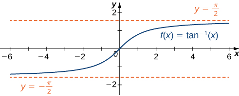
Figure \(\PageIndex{6}\): This function has two horizontal asymptotes.

This limit can be useful enough, that it is good to formalize it in a theorem along with some other common limits.

Theorem \(\PageIndex{3}\)

\[ \lim_{x \to \infty}{\tan^{−1}{(x)}} = \frac{\pi}{2}, \nonumber \]

\[ \lim_{x \to -\infty}{\tan^{−1}{(x)}} = −\frac{\pi}{2}, \nonumber\]

\[ \lim_{x \to \infty}{\tanh{(x)}} = 1, \nonumber\]

\[ \lim_{x \to -\infty}{\tanh{(x)}} = -1, \text{ and }\nonumber\]

\[ \lim_{x \to \infty}{b^{-x}} = 0, \text{ where }b \gt 1. \nonumber\]

---

Revisiting the Squeeze Theorem

We have already seen that a lot of our original theory of finite limits at finite numbers can be applied to finite limits at infinity. We round out this collection of common theorems by revisiting the Squeeze Theorem.

Theorem \(\PageIndex{4}\): The Squeeze Theorem for Limits at Infinity

Let \(f(x),g(x)\), and \(h(x)\) be defined for all \(x \gt a\), where \(a\) is a real number. If

\[f(x) \leq g(x) \leq h(x) \nonumber \]

for all \(x \gt a\) and

\[\lim_{x \to \infty}f(x)=L=\lim_{x \to \infty}h(x) \nonumber \]

where \(L\) is a real number, then \(\displaystyle \lim_{x \to \infty}g(x)=L.\)

Likewise, let \(f(x),g(x)\), and \(h(x)\) be defined for all \(x \lt a\), where \(a\) is a real number. If

\[f(x) \leq g(x) \leq h(x) \nonumber \]

for all \(x \lt a\) and

\[\lim_{x \to -\infty}f(x)=L=\lim_{x \to -\infty}h(x) \nonumber \]

where \(L\) is a real number, then \(\displaystyle \lim_{x \to -\infty}g(x)=L.\)

Example \(\PageIndex{4}\)

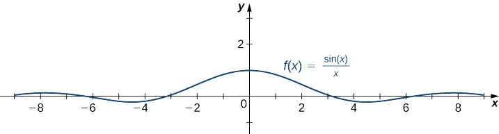
Evaluate \(\displaystyle \lim_{x \to \infty}{\dfrac{\sin{(x)}}{x}}\) and \(\displaystyle \lim_{x \to -\infty}{\dfrac{\sin{(x)}}{x}}\). Determine the horizontal asymptote(s) for \(f(x) = \frac{\sin{(x)}}{x}\).

Solution

Since \(-1 \leq \sin x \leq 1\) for all \(x\), we have

\[\frac{−1}{x} \leq \frac{\sin x}{x} \leq \frac{1}{x}\nonumber \]

for all \(x \neq 0\). Also, since

\(\displaystyle \lim_{x \to \infty}\frac{−1}{x}=0=\lim_{x \to \infty}\frac{1}{x}\),

we can apply the Squeeze Theorem to conclude that

\(\displaystyle \lim_{x \to \infty}\frac{\sin x}{x}=0.\)

Similarly,

\(\displaystyle \lim_{x \to −\infty}\frac{\sin x}{x}=0.\)

Thus, \(f(x)=\dfrac{\sin x}{x}\) has a horizontal asymptote of \(y=0\) and \(f(x)\) approaches this horizontal asymptote as \(x \to \pm \infty\) as shown in the following graph.

Figure \(\PageIndex{7}\): This function crosses its horizontal asymptote multiple times.

---

Infinite Limits at Infinity

Sometimes the values of a function \(f\) become arbitrarily large as \(x \to \infty \) (or as \(x \to −\infty\)). In this case, we write \(\displaystyle \lim_{x \to \infty}f(x)=\infty\) (or \(\displaystyle \lim_{x \to −\infty}f(x)=\infty\)). On the other hand, if the values of \(f\) are negative but become arbitrarily large in magnitude as \(x \to \infty\) (or as \(x \to −\infty\)), we write \(\displaystyle \lim_{x \to \infty}f(x)=−\infty\) (or \(\displaystyle \lim_{x \to −\infty}f(x)=−\infty\)).

For example, consider the function \(f(x)=x^3\). As seen in Table \(\PageIndex{2}\) and Figure \(\PageIndex{8}\), as \(x \to \infty\) the values \(f(x)\) become arbitrarily large. Therefore, \(\displaystyle \lim_{x \to \infty}x^3=\infty\). On the other hand, as \(x \to −\infty\), the values of \(f(x)=x^3\) are negative but become arbitrarily large in magnitude. Consequently, \(\displaystyle \lim_{x \to −\infty}x^3=−\infty.\)

Table \(\PageIndex{2}\): Values of a power function as \(x \to \pm \infty\)

\(x\)	10	20	50	100	1000
\(x^3\)	1000	8000	125,000	1,000,000	1,000,000,000
\(x\)	−10	−20	−50	−100	−1000
\(x^3\)	−1000	−8000	−125,000	−1,000,000	−1,000,000,000

 
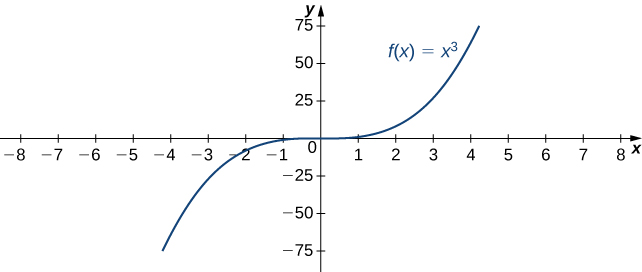
Figure \(\PageIndex{8}\): For this function, the functional values approach \( \pm \)infinity as \(x \to \pm \infty.\)

Definition: Infinite Limit at Infinity (Informal)

We say a function \(f\) has an infinite limit at infinity and write

\[\lim_{x \to \infty}f(x)=\infty. \nonumber \]

if \(f(x)\) becomes arbitrarily large for \(x\) sufficiently large. We say a function has a negative infinite limit at infinity and write

\[\lim_{x \to \infty}f(x)=−\infty. \nonumber \]

if \(f(x)<0\) and \(|f(x)|\) becomes arbitrarily large for \(x\) sufficiently large. Similarly, we can define infinite limits as \(x \to −\infty.\) 

In general, infinite limits at infinity require fewer prerequisite manipulations to evaluate than other types of limits, and require more conceptual investigation. The following theorem (which will will prove parts of in the next section) contains some very common infinite limits at infinity.

Theorem \(\PageIndex{5}\)

• \( \displaystyle \lim_{x \to \infty} x = \infty \)
• \( \displaystyle \lim_{x \to -\infty} x = -\infty \)
• If \( p \gt 0 \), \( \displaystyle \lim_{x \to \infty} x^p = \infty \)
• If \( b > 1 \), \( \displaystyle \lim_{x \to \infty} b^x = \infty. \)

Example \(\PageIndex{5}\): Evaluating an Infinite Limit at Infinity

Evaluate the limit

\[ \lim_{x \to -\infty}{ \frac{3 + x^6}{x^4 + 8} } \nonumber \]

Solution

\[ \begin{array}{rcll} \displaystyle \lim_{x \to -\infty}{ \frac{3 + x^6}{x^4 + 8} } & = & \displaystyle \lim_{x \to -\infty}{ \frac{\frac{3}{x^6} + 1}{\frac{1}{x^2} + \frac{8}{x^6}} } & (\text{Algebra: divide numerator and denominator by }x^6) \\ \end{array} \nonumber \]

Since \(3/x^6 \to 0\) as \(x \to -\infty\), we know the numerator is approaching \(1\). Moreover, as \(x \to -\infty\),

\[ \frac{1}{x^2} + \frac{8}{x^6} \to 0^+ + 0^+ \to 0^+ \nonumber \]

Hence, 

\[ \lim_{x \to -\infty}{ \frac{3 + x^6}{x^4 + 8} } = \infty. \nonumber \]

---

Key Concepts

• The limit of \(f(x)\) is \(L\) as \(x \to \infty\) (or as \(x \to −\infty)\) if the values \(f(x)\) become arbitrarily close to \(L\) as \(x\) becomes sufficiently large.
• The limit of \(f(x)\) is \(\infty\) as \(x \to \infty\) if \(f(x)\) becomes arbitrarily large as \(x\) becomes sufficiently large. The limit of \(f(x)\) is \(−\infty\) as \(x \to \infty\) if \(f(x)<0\) and \(|f(x)|\) becomes arbitrarily large as \(x\) becomes sufficiently large. We can define the limit of \(f(x)\) as \(x\) approaches \(−\infty\) similarly.

---

Common Mistakes

• Prerequisite Mistakes
  • Bad factoring
  • Not understanding conjugate multiplication
  • Not knowing the graphs of prerequisite algebraic and transcendental functions
  • Not understanding how to handle \(\sqrt[n]{x^n}\)
• Using the Limit Laws on functions whose limits are not finite
• Using a table to estimate the value of a limit
• Not understanding that when the limit is indeterminate of the form \(\infty/\infty\) or \(\infty - \infty\), algebraic manipulations must be performed (we will learn a different technique to handle these types of limits later in the course).

---

Glossary

end behavior

the behavior of a function as \(x \to \infty\) and \(x \to −\infty\)

finite limit at infinity

a function that approaches a limit value \(L\) as \(x\) becomes large

horizontal asymptote

if \(\displaystyle \lim_{x \to \infty}f(x)=L\) or \(\displaystyle \lim_{x \to −\infty}f(x)=L\), then \(y=L\) is a horizontal asymptote of \(f\)

infinite limit at infinity

a function that becomes arbitrarily large as \(x\) becomes large