3.5: Derivatives of Exponential and Hyperbolic Functions

Learning Objectives

• Find the derivative of exponential functions, both natural-based and non-natural-based.
• Find the derivative of logarithmic functions, both natural-based and non-natural-based.
• Apply the formulas for derivatives of the hyperbolic functions.
• Explore applications for the derivatives of exponential and hyperbolic functions in the sciences and engineering.

So far, we have learned how to differentiate a variety of functions, including polynomial, radical, rational, and trigonometric functions. In this section, we explore derivatives of exponential and hyperbolic functions.

Discovering \(e\)

In calculus (and often in precalculus), a common "beginning" limit to investigate numerically is

\[ \displaystyle \lim_{k \to \infty}{\left(1 + \frac{1}{k}\right)^k}. \nonumber \]

Table \(\PageIndex{1}\) shows values of this limit for large values of \(k\).

Table \(\PageIndex{1}\): Investigating a Famous Limit

\(k\)	\(\left(1 + \frac{1}{k}\right)^k\)
10	2.5937424601...
100	2.70481382942153...
1,000	2.71692393223552...
10,000	2.71814592682436...
100,000	2.71826823719753...
1,000,000	2.71828046915643...
10,000,000	2.71828169398037...
100,000,000	2.71828178639580...
1,000,000,000	2.71828203081451...

We went a little overboard, but you get the point. It appears this limit is approaching some value around \(2.71828\ldots\). This very special value is a non-terminating, non-repeating number. That is, it is an irrational number - just like \(\pi\). In fact, if we could assign an importance to the value of this limit, it would be tied with the importance of the numbers \(0\), \(1\), \(\pi\), and \(i = \sqrt{-1}\).

This limit comes up so often in the sciences that we give it a special name. Rather than calling it, "the limit that approaches \(2.718281828459045\ldots\)," we call it \(e\). As was mentioned, it appears via our table that this limit approaches a constant (that we are deciding to label \(e\)); however, the proof of this fact is reserved for later in the course. For now, it's important to have this limit in hand for use.

An important alternative form for this limit is found by letting \(n = \frac{1}{k}\). As \(k \to \infty\), \(n \to 0\) and we get the form

\[ \displaystyle \lim_{n \to 0}{\left(1 + n\right)^{1/n}}. \nonumber \]

Before we move on, let's formalize this definition.

Definition: \(e\)

The limit

\[ \displaystyle \lim_{k \to \infty}{\left(1 + \frac{1}{k}\right)^k} = \displaystyle \lim_{n \to 0}{\left(1 + n\right)^{1/n}} \nonumber \]

is defined to be the irrational number \(e\).

Fear not, we will be using this special number shortly; however, before we do, we need to discuss some Calculus. 

Derivatives Exponential Functions

Just as when we found the derivatives of other functions, we can find the derivatives of exponential functions using formulas. Recall that all non-transformed exponential functions have the basic form \(B(x) = b^x\), where \(b \gt 0\) and \(b \neq 1\). Our initial goal is to prove that exponential functions are continuous everywhere. Once we have this, the proof of the derivative of an exponential function becomes trivial.

Proving that Exponential Functions are Continuous Everywhere

In previous courses, the values of exponential functions for all rational numbers were defined. We began with the definition of \(b^n\), where \(n \in \mathbb{N}\), as the product of \(b\) multiplied by itself \(n\) times. Later, we defined \(b^0=1\) , \(b^{−n}=\frac{1}{b^n}\) for \(n \in \mathbb{N}\), and \(b^{s/t}=(\sqrt[t]{b})^s\) for positive integers \(s\) and \(t\). These definitions define exponential functions over the rational numbers, but leave open the question of the value of \(b^r\) where \(r\) is an irrational number.

By assuming the continuity of \(B(x)=b^x,b>0\), we may interpret \(b^r\) as \(\displaystyle \lim_{x \to r}b^x\) where the values of \(x\) as we take the limit are rational. For example, we may view \(4^ \pi \) as the number satisfying

\[ \begin{array}{rcccl}
4^3 & < & 4^ \pi & < & 4^4 \\
4^{3.1} & < & 4^ \pi & < & 4^{3.2} \\
4^{3.14} & < & 4^ \pi & < & 4^{3.15} \\
4^{3.141} & < & 4^{ \pi } & < & 4^{3.142} \\
4^{3.1415} & < & 4^{ \pi } & < & 4^{3.1416} \\
& & \vdots & & \\
\end{array} \nonumber \]

As we see in the following table, \(4^ \pi \approx 77.88.\)

\(x\)	\(4^x\)	\(x\)	\(4^x\)
\(4^3\)	64	\(4^{3.141593}\)	77.8802710486
\(4^{3.1}\)	73.5166947198	\(4^{3.1416}\)	77.8810268071
\(4^{3.14}\)	77.7084726013	\(4^{3.142}\)	77.9242251944
\(4^{3.141}\)	77.8162741237	\(4^{3.15}\)	78.7932424541
\(4^{3.1415}\)	77.8702309526	\(4^{3.2}\)	84.4485062895
\(4^{3.14159}\)	77.8799471543	\(4^{4}\)	256

Approximating a Value of \(4^ \pi \)

To prove that the exponential function \(B(x) = b^x\) is continuous on \(\mathbb{R}\), we need to first prove that \( B(x) = b^x \) is continuous at \( x = 0 \).

Proof that \( B(x) = b^x \) is continuous at \( x = 0 \)

Suppose \( x \gt 0 \). \( \forall \epsilon \gt 0 \), if we choose \( \delta = \log_b(1 + \epsilon) \), then

\[ \begin{array}{rccccll}
& 0 & \lt & |x - 0| & \lt & \delta & \\
\implies &  &  & x & \lt & \delta & \left( x \gt 0 \implies |x| = x \right) \\
\implies &  &  & x & \lt & \log_b(1 + \epsilon) & \\
\implies &  &  & b^x & \lt & 1 + \epsilon & \\
\implies &  &  & b^x - 1 & \lt & \epsilon & \\
\implies &  &  & |b^x - 1| & \lt & \epsilon & \left( x \gt 0 \implies b^x \gt b^0 = 1 \implies b^x - 1 \gt 0 \implies b^x - 1 = |b^x - 1| \right) \\
\end{array} \nonumber \]

Therefore, \( \displaystyle \lim_{x \to 0^+} b^x = 1 = b^0 \). 

Moreover, if \( x \lt 0 \), then \( \forall \epsilon \gt 0 \), we choose \( \delta = -\log_b(1 - \epsilon) \). Therefore,

\[ \begin{array}{rccccll}
& 0 & \lt & |x - 0| & \lt & \delta & \\
\implies &  &  & -x & \lt & \delta & \left( x \lt 0 \implies |x| = -x \right) \\
\implies &  &  & -x & \lt & -\log_b(1 - \epsilon) & \\
\implies &  &  & x & \gt & \log_b(1 - \epsilon) & \\
\implies &  &  & b^x & \gt & 1 - \epsilon & \\
\implies &  &  & b^x - 1 & \gt & -\epsilon & \\
\implies &  &  & -(b^x - 1) & \lt & \epsilon & \\
\implies &  &  & |b^x - 1| & \lt & \epsilon & \left( x \lt 0 \implies b^x \lt b^0 = 1 \implies b^x - 1 \lt 0 \implies -(b^x - 1) = |b^x - 1| \right) \\
\end{array} \nonumber \]

Therefore, \( \displaystyle \lim_{x \to 0^-} b^x = 1 = b^0 \). 

Since both one-sided limits are equal to \( b^0 \), \( \displaystyle \lim_{x \to 0} b^x = 1 = b^0 \). Thus, \( B(x) = b^x \) is continuous at \( x = 0 \).

We are now ready to prove that \( B(x) = b^x \) is continuous everywhere.

Let \(B(x) = b^x\) and let \(a\) be arbitrary. Then

\[ \begin{array}{rclr}
\displaystyle \lim_{x \to a}{b^x} & = & \displaystyle \lim_{h \to 0}{b^{a + h}} & \left(\text{Substitution: let }x = a + h \implies h = x - a\text{. Thus, }h \to 0\text{ as }x \to a\right) \\
 & = & \displaystyle \lim_{h \to 0}{\left( b^a \cdot b^h \right)} & \\
 & = & \displaystyle b^a \cdot \lim_{h \to 0}{b^h} &  \left(\text{Calculus: Constant Multiple Limit Law}\right) \\
 & = & \displaystyle b^a \cdot b^0 & \left(\text{Calculus: }b^x\text{ is continuous at }0 \right) \\
 & = & \displaystyle b^a  &  \\
\end{array} \nonumber \]

Since \(a\) is arbitrary, this shows that the exponential function \(B(x) = b^x\) is continuous everywhere.

The next theorem is a fascinating fact, and is the student's favorite derivative. In words, the function \(y = e^x\) is the only function (besides \(y = 0\)) whose derivative is itself!

Theorem \(\PageIndex{1}\): Derivative of \(e^x\)

\[ \dfrac{d}{dx}\left(e^x\right) = e^x \nonumber \]

Proof

Using the limit definition of the derivative, we get the following:

\[ \begin{array}{rclr}
\dfrac{d}{dx} \left( e^x \right) & = & \displaystyle \lim_{h \to 0}{ \dfrac{e^{x + h} - e^x}{h} } & \left(\text{Calculus: definition of a derivative}\right) \\
 & = & \displaystyle \lim_{h \to 0}{ \dfrac{e^x \cdot e^h - e^x}{h} } &  \\
 & = & \displaystyle \lim_{h \to 0}{ \dfrac{e^x \left(e^h - 1\right)}{h} } & \\
 & = & \displaystyle e^x \cdot \lim_{h \to 0}{ \dfrac{e^h - 1}{h} } & \left(\text{Calculus: since }e^x\text{ does not rely on }h\text{, it can be factored out}\right) \\
\end{array} \nonumber \]

Recall that we defined \(e\) to be \( \displaystyle \lim_{n \to \infty}{\left(1 + n\right)^{1/n}} \). If we let \(n = e^h - 1\), then \(n + 1 = e^h\). Since exponential functions are continuous everywhere,

\[ \displaystyle \lim_{h \to 0}{e^h} = e^0 = 1. \nonumber \]

This means that \(n \to 0\) as \(h \to 0\). Moreover, solving \(n + 1 = e^h\) for \(h\), we get \(\ln{(n+1)} = h\). Thus,

\[ \begin{array}{rclr}
\dfrac{d}{dx} \left( e^x \right) & = & \displaystyle e^x \cdot \lim_{h \to 0}{ \dfrac{e^h - 1}{h} } & \\
 & = & \displaystyle e^x \cdot \lim_{n \to 0}{ \dfrac{n}{\ln{(1 + n)}} } &  \\
 & = & \displaystyle e^x \cdot \lim_{n \to 0}{ \dfrac{1}{\frac{1}{n}\ln{(1 + n)}} } & \\
 & = & \displaystyle e^x \cdot \lim_{n \to 0}{ \dfrac{1}{\ln{(1 + n)^{1/n}}} } & \\
 & = & e^x \cdot \dfrac{1}{\displaystyle \lim_{n \to 0}{\ln{(1 + n)^{1/n}}}} & \left(\text{Calculus: Limit Laws}\right) \\
 & = & e^x \cdot \dfrac{1}{\ln{\left( \displaystyle \lim_{n \to 0}{(1 + n)^{1/n}}\right)}} & \left(\text{Calculus: Limit Laws}\right) \\
 & = & e^x \cdot \dfrac{1}{\ln{(e)}} & \left(\text{Definition of }e\right) \\
 & = & e^x \cdot \dfrac{1}{1} & \\
 & = & e^x & \\
\end{array} \nonumber \]

Q.E.D.

Before going into examples, let's add a quick corollary.

Corollary \(\PageIndex{1}\): Derivative of \(b^x\)

\[ \dfrac{d}{dx}\left(b^x\right) = b^x \ln{(b)} \nonumber \]

Proof

\[ \begin{array}{rclr}
\dfrac{d}{dx}\left( b^x \right) & = & \dfrac{d}{dx}\left( e^{\ln{\left(b^x \right)}}\right) & \\
 & = & \dfrac{d}{dx}\left( e^{x \ln{(b)}}\right) & \\
 & = & e^{x \ln{(b)}} \cdot \ln{(b)} & \left(\text{Calculus: Chain Rule}\right) \\
 & = & e^{\ln{(b^x)}} \cdot \ln{(b)} & \\
 & = & b^x \cdot \ln{(b)} & \\
\end{array} \nonumber \]

Q.E.D.

Example \(\PageIndex{1}\): Derivative of an Exponential Function

Find the derivative of \(f(x)=e^{\tan(2x)}\).

Solution

Using the derivative formula and the Chain Rule,

\[f^{\prime}(x)=e^{\tan(2x)}\frac{d}{dx}\Big(\tan(2x)\Big)=e^{\tan(2x)}\sec^2(2x) \cdot 2 \nonumber \]

Example \(\PageIndex{2}\): Combining Differentiation Rules

Find the derivative of \(y=\frac{e^{x^2}}{x}\).

Solution

Use the derivative of the natural exponential function, the Quotient Rule, and the Chain Rule.

\[\begin{array}{rclr}
y^{\prime} & = & \dfrac{(e^{x^2} \cdot 2)x \cdot x−1 \cdot e^{x^2}}{x^2} & \left( \text{Apply the Quotient Rule.} \right) \\
& = & \dfrac{e^{x^2}(2x^2−1)}{x^2} & \\
\end{array}\nonumber\]

Exercise \(\PageIndex{2}\)

Find the derivative of \(h(x)=xe^{2x}\).

Hint

Don’t forget to use the Product Rule.

Answer

\(h^{\prime}(x)=e^{2x}+2xe^{2x}\)

Example \(\PageIndex{3}\): Applying the Natural Exponential Function

A colony of mosquitoes has an initial population of 1000. After \(t\) days, the population is given by \(A(t)=1000e^{0.3t}\). Show that the ratio of the rate of change of the population, \(A^{\prime}(t)\), to the population, \(A(t)\) is constant.

Solution

First find \(A^{\prime}(t)\). By using the Chain Rule, we have \(A^{\prime}(t)=300e^{0.3t}.\) Thus, the ratio of the rate of change of the population to the population is given by

\[\frac{A^{\prime}(t)}{A(t)}=\dfrac{300e^{0.3t}}{1000e^{0.3t}}=0.3. \nonumber \]

The ratio of the rate of change of the population to the population is the constant 0.3.

Exercise \(\PageIndex{3}\)

If \(A(t)=1000e^{0.3t}\) describes the mosquito population after \(t\) days, as in the preceding example, what is the rate of change of \(A(t)\) after 4 days?

Hint

Find \(A^{\prime}(4)\).

Answer

\(996\)

Example \(\PageIndex{4}\): Applying Derivative Formulas

Find the derivative of \(h(x)=\frac{3^x}{3^x+2}\).

Solution

\[\begin{array}{rclr}
h^{\prime}(x) & = & \dfrac{3^x\ln 3(3^x+2)−3^x\ln 3(3^x)}{(3^x+2)^2} & \left( \text{Apply the Quotient Rule.} \right) \\
& = & \dfrac{2 \cdot 3^x\ln 3}{(3x+2)^2} & \\
\end{array} \nonumber\]

Exercise \(\PageIndex{4}\)

Find the slope for the line tangent to \(y=3^x\) at \(x=2.\)

Hint

Evaluate the derivative at \(x=2.\)

Answer

\(9\ln(3)\)

Derivatives of the Hyperbolic Functions

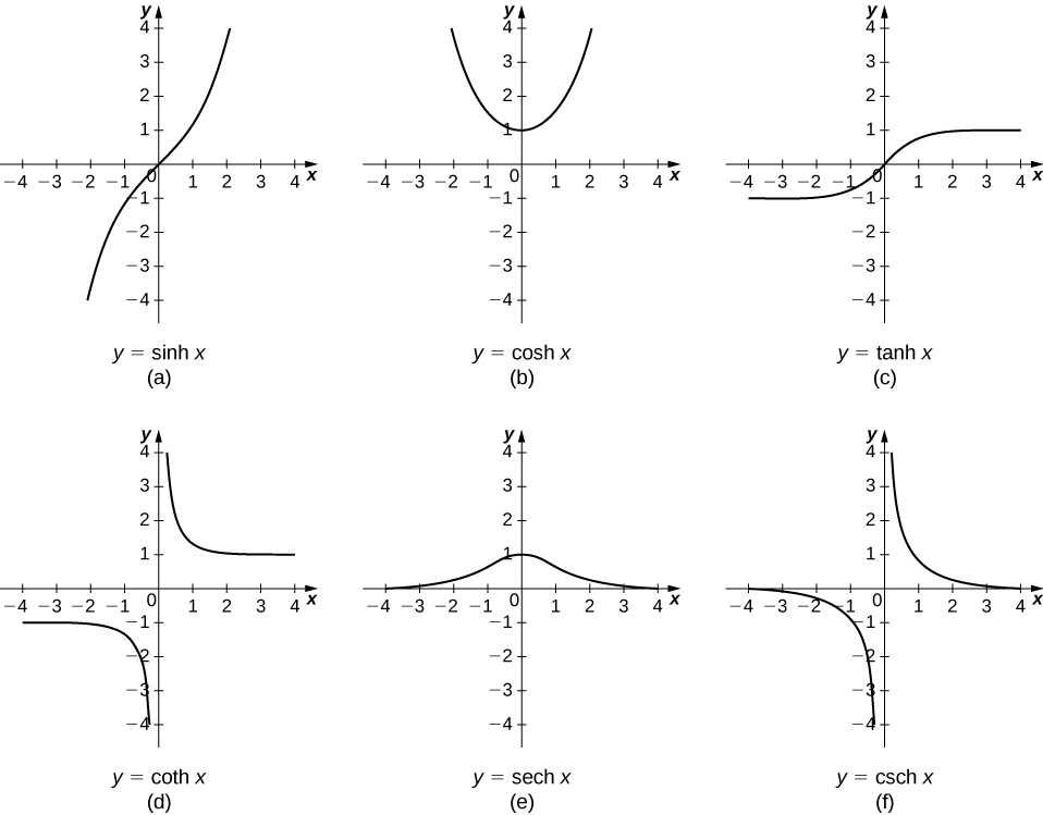
Recall that the hyperbolic sine and hyperbolic cosine are defined as

\[\sinh x=\dfrac{e^x−e^{−x}}{2} \nonumber \]

and

\[\cosh x=\dfrac{e^x+e^{−x}}{2}. \nonumber \]

The other hyperbolic functions are then defined in terms of \(\sinh x\) and \(\cosh x\). The graphs of the hyperbolic functions are shown in Figure \(\PageIndex{1}\).

Figure \(\PageIndex{1}\): Graphs of the hyperbolic functions.

It is easy to develop differentiation formulas for the hyperbolic functions. For example, looking at \(\sinh x\) we have

\[\begin{array}{rcl}
\dfrac{d}{dx} \left(\sinh x \right) & = & \dfrac{d}{dx} \left(\dfrac{e^x−e^{−x}}{2}\right) \\
& = & \dfrac{1}{2}\left[\dfrac{d}{dx}(e^x)−\dfrac{d}{dx}(e^{−x})\right] \\
& = & \dfrac{1}{2}[e^x+e^{−x}] \\
& = \cosh x. \\
\end{array} \nonumber \]

Similarly,

\[\dfrac{d}{dx} \cosh x=\sinh x. \nonumber \]

We summarize the differentiation formulas for the hyperbolic functions in Table \(\PageIndex{2}\).

Table \(\PageIndex{2}\): Derivatives of the Hyperbolic Functions

\(f(x)\)	\(\dfrac{d}{dx}f(x)\)
\(\sinh x\)	\(\cosh x\)
\(\cosh x\)	\(\sinh x\)
\(\tanh x\)	\(\text{sech}^2 \,x\)
\(\text{coth } x\)	\(−\text{csch}^2\, x\)
\(\text{sech } x\)	\(−\text{sech}\, x \tanh x\)
\(\text{csch } x\)	\(−\text{csch}\, x \coth x\)

Let’s take a moment to compare the derivatives of the hyperbolic functions with the derivatives of the standard trigonometric functions. There are a lot of similarities, but differences as well. For example, the derivatives of the sine functions match:

\[\dfrac{d}{dx} \sin x=\cos x \nonumber \]

and

\[\dfrac{d}{dx} \sinh x=\cosh x. \nonumber \]

The derivatives of the cosine functions, however, differ in sign:

\[\dfrac{d}{dx} \cos x=−\sin x, \nonumber \]

but

\[\dfrac{d}{dx} \cosh x=\sinh x. \nonumber \]

Example \(\PageIndex{5}\)

Evaluate the following derivatives:

1. \(\frac{d}{dx}(\sinh(x^2))\)
2. \(\frac{d}{dx}(\cosh x)^2\)

Solution

Using the formulas in Table \(\PageIndex{2}\) and the Chain Rule, we get

1.  
   \[\dfrac{d}{dx}(\sinh(x^2))=\cosh(x^2) \cdot 2x\nonumber\]
2. 
   \[\dfrac{d}{dx}(\cosh x)^2=2\cosh x\sinh x\nonumber\]

Exercise \(\PageIndex{6}\)

Evaluate the following derivatives:

1. \(\frac{d}{dx}(\tanh(x^2+3x))\)
2. \(\frac{d}{dx}\left(\frac{1}{(\sinh x)^2}\right)\)

Hint

Use the formulas in Table \(\PageIndex{2}\) and apply the Chain Rule as necessary.

Answer a

\(\frac{d}{dx}(\tanh(x^2+3x))=(\text{sech}^2(x^2+3x))(2x+3)\)

Answer b

\(\frac{d}{dx}\left(\frac{1}{(\sinh x)^2}\right)=\frac{d}{dx}(\sinh x)^{−2}=−2(\sinh x)^{−3}\cosh x\)

Key Concepts

• On the basis of the assumption that the exponential function \(y=b^x, \,b>0\) is continuous everywhere and differentiable at \(0\), this function is differentiable everywhere and there is a formula for its derivative.
• We can use a formula to find the derivative of \(y=\ln x\), and the relationship \(\log_b x=\dfrac{\ln x}{\ln b}\) allows us to extend our differentiation formulas to include logarithms with arbitrary bases.
• Logarithmic differentiation allows us to differentiate functions of the form \(y=g(x)^{f(x)}\) or very complex functions by taking the natural logarithm of both sides and exploiting the properties of logarithms before differentiating.
• Hyperbolic functions are defined in terms of exponential functions.
• Term-by-term differentiation yields differentiation formulas for the hyperbolic functions. These differentiation formulas give rise, in turn, to integration formulas.
• With appropriate range restrictions, the hyperbolic functions all have inverses.
• Implicit differentiation yields differentiation formulas for the inverse hyperbolic functions, which in turn give rise to integration formulas.
• The most common physical applications of hyperbolic functions are calculations involving catenaries.

Key Equations

• Derivative of the natural exponential function

\(\dfrac{d}{dx}\Big(e^{g(x)}\Big)=e^{g(x)}g′(x)\)

• Derivative of the natural logarithmic function

\(\dfrac{d}{dx}\Big(\ln g(x)\Big)=\dfrac{1}{g(x)}g′(x)\)

• Derivative of the general exponential function

\(\dfrac{d}{dx}\Big(b^{g(x)}\Big)=b^{g(x)}g′(x)\ln b\)

• Derivative of the general logarithmic function

\(\dfrac{d}{dx}\Big(\log_b g(x)\Big)=\dfrac{g′(x)}{g(x)\ln b}\)

Glossary

catenary

a curve in the shape of the function \(y=a\cdot\cosh(x/a)\) is a catenary; a cable of uniform density suspended between two supports assumes the shape of a catenary

logarithmic differentiation

is a technique that allows us to differentiate a function by first taking the natural logarithm of both sides of an equation, applying properties of logarithms to simplify the equation, and differentiating implicitly