3.7: Derivatives of Logarithmic, Inverse Trigonometric, and Inverse Hyperbolic Functions

Learning Objectives

• Compute the derivative of a logarithmic function, both natural-based and non-natural-based.
• Calculate the derivative of an inverse trigonometric function.
• Recognize the derivatives of the inverse hyperbolic functions.

Now that we have the Chain Rule and implicit differentiation under our belts, we can explore the derivatives of logarithmic functions as well as the relationship between the derivative of a function and the derivative of its inverse. For functions whose derivatives we already know, we can use this relationship to find derivatives of inverses without having to use the limit definition of the derivative. In particular, we will apply the formula for derivatives of inverse functions to trigonometric functions. This formula may also be used to extend the Power Rule to rational exponents.

Derivative of the Logarithmic Function

Now that we have the derivative of the natural exponential function, we can use implicit differentiation to find the derivative of its inverse, the natural logarithmic function.

Theorem \(\PageIndex{1}\): The Derivative of the Natural Logarithmic Function

If \(y=\ln x\), then

\[\frac{dy}{dx}=\frac{1}{x}. \nonumber \]

Proof

If \(y=\ln x\), then \(e^y=x.\) Differentiating both sides of this equation results in the equation

\[e^y\frac{dy}{dx}=1. \nonumber \]

Solving for \(\dfrac{dy}{dx}\) yields

\[\frac{dy}{dx}=\frac{1}{e^y}. \nonumber \]

Finally, we substitute \(x=e^y\) to obtain

\[\frac{dy}{dx}=\frac{1}{x}. \nonumber \]

Q.E.D.

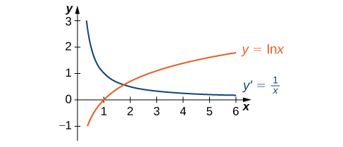
The graph of \(y=\ln x\) and its derivative \(\dfrac{dy}{dx}=\dfrac{1}{x}\) are shown in Figure \(\PageIndex{1}\).

Figure \(\PageIndex{1}\): The function \(y=\ln x\) is increasing on \((0,+ \infty)\). Its derivative \(y'=\frac{1}{x}\) is greater than zero on \((0,+ \infty)\)

Example \(\PageIndex{1}\): Taking a Derivative of a Natural Logarithm

Find the derivative of \(f(x)=\ln(x^3+3x−4)\).

Solution

\[ \begin{array}{rclr}
f^{\prime}(x) & = & \dfrac{1}{x^3+3x−4} \cdot \dfrac{d}{dx} \left(x^3 + 3x - 4\right) & \left(\text{Calculus: Chain Rule}\right) \\
 & = & \dfrac{1}{x^3+3x−4} \cdot \left(3x^2 + 3\right) & \\
 & = & \dfrac{3x^2 + 3}{x^3+3x−4} & \\
 & = & \dfrac{3(x^2 + 1)}{x^3+3x−4} & \\
\end{array} \nonumber \]

As an aside, it is always a good idea to clean up derivatives using our prerequisite algebra. Sometimes things clean up very nicely.

Example \(\PageIndex{2}\): Using Properties of Logarithms in a Derivative

Find the derivative of \(f(x)=\ln\left(\frac{x^2\sin x}{2x+1}\right)\).

Solution

At first glance, taking this derivative appears rather complicated. However, by using the properties of logarithms prior to finding the derivative, we can make the problem much simpler.

\[f(x) = \ln\left(\frac{x^2\sin x}{2x+1}\right) = 2\ln x+\ln(\sin x)−\ln(2x+1)\nonumber\]

Hence,

\[\begin{array}{rclr}
f^{\prime}(x) & = & \dfrac{2}{x} + \dfrac{1}{\sin x} \cdot \cos x − \dfrac{1}{2x+1} \cdot 2 & \left( \text{Derivative of the natural log and the Chain Rule.} \right) \\
& = & \dfrac{2}{x} + \cot x − \dfrac{2}{2x+1} & \\
 \end{array}\nonumber\]

Exercise \(\PageIndex{2}\)

Differentiate: \(f(x)=\ln(3x+2)^5\).

Hint

Use a property of logarithms to simplify before taking the derivative.

Answer

\(f^{\prime}(x)=\frac{15}{3x+2}\)

Now that we can differentiate the natural logarithmic function, we can use this result to find the derivatives of \(y=\log_b x\) for \(b>0, \,b \neq 1\).

Theorem \(\PageIndex{2}\): The General Derivative of a Logarithmic Function

\[ \dfrac{d}{dx} \left( \log_{b}{(x)} \right) = \dfrac{1}{x \ln{(b)}} \nonumber \]

Proof

If \(y=\log_b x,\) then \(b^y=x.\) It follows that \(\ln(b^y)=\ln x\). Thus \(y\ln b=\ln x\). Solving for \(y\), we have \(y=\frac{\ln x}{\ln b}\). Differentiating and keeping in mind that \(\ln b\) is a constant, we see that

\[\frac{dy}{dx}=\frac{1}{x\ln b}. \nonumber \]

Q.E.D.

Example \(\PageIndex{3}\): Finding the Slope of a Tangent Line

Find the slope of the line tangent to the graph of \(y=\log_2 (3x+1)\) at \(x=1\).

Solution

To find the slope, we must evaluate \(\frac{dy}{dx}\) at \(x=1\).

\[\dfrac{dy}{dx}=\dfrac{3}{(3x+1)\ln 2}. \nonumber \]

By evaluating the derivative at \(x=1\), we see that the tangent line has slope

\[\dfrac{dy}{dx}\bigg{|}_{x=1}=\dfrac{3}{4\ln 2}=\dfrac{3}{\ln 16}. \nonumber \]

Aside: Revisiting the Generalized Power Rule

We now have enough "mathematical prowess" to continue our proof of the Generalized Power Rule from earlier in this chapter. This time, we add the ability to take the derivative of \(y = x^n\), where \(n\) is a rational number.

Proof

Let \(y = x^n\), where \(n\) is a rational number. Then \(n\) can be written as \(p/q\), for integers \(p\) and \(q\).

\[ \begin{array}{rclcrcl}
y & = & x^n & \implies & y & = & x^{p/q} \\
 & &  & \implies & y^q & = & x^p \\
 & &  & \implies & \dfrac{d}{dx} \left( y^q \right) & = & \dfrac{d}{dx} \left( x^p \right) \\
 & &  & \implies & q y^{q - 1} \dfrac{dy}{dx} & = & p x^{p - 1} \\
 & &  & \implies & \dfrac{dy}{dx} & = & \dfrac{p x^{p - 1}}{q y^{q - 1}} \\
 & &  & \implies & \dfrac{dy}{dx} & = & \dfrac{p}{q} \cdot \dfrac{x^{p - 1}}{y^{q - 1}} \\
 & &  & \implies & \dfrac{dy}{dx} & = & \dfrac{p}{q} \cdot \dfrac{x^{p - 1}}{\left(x^{p/q}\right)^{q - 1}} \\
 & &  & \implies & \dfrac{dy}{dx} & = & \dfrac{p}{q} \cdot \dfrac{x^{p - 1}}{x^{p - p/q}} \\
 & &  & \implies & \dfrac{dy}{dx} & = & \dfrac{p}{q} \cdot x^{p/q - 1} \\
 & &  & \implies & \dfrac{dy}{dx} & = & n  x^{n - 1} \\
\end{array}
\nonumber \]

Q.E.D.

Derivatives of Inverse Trigonometric Functions

We now turn our attention to finding derivatives of inverse trigonometric functions. These derivatives will prove invaluable in the study of integration later in this text. The derivatives of inverse trigonometric functions are quite surprising in that their derivatives are actually algebraic functions. Previously, derivatives of algebraic functions have proven to be algebraic functions and derivatives of trigonometric functions have been shown to be trigonometric functions. Here, for the first time, we see that the derivative of a function need not be of the same type as the original function.

Theorem \(\PageIndex{3}\): Derivatives of the Inverse Trigonometric Functions

\[ \begin{array}{rclcrcl}
\dfrac{d}{dx}\big(\sin^{−1}x\big) & = & \dfrac{1}{\sqrt{1−x^2}} & \quad & \dfrac{d}{dx}\big(\csc^{−1}x\big) & = & -\dfrac{1}{x \sqrt{x^2−1}} \\
\dfrac{d}{dx}\big(\cos^{−1}x\big) & = & -\dfrac{1}{\sqrt{1−x^2}} & \quad & \dfrac{d}{dx}\big(\sec^{−1}x\big) & = & \dfrac{1}{x \sqrt{x^2−1}} \\
\dfrac{d}{dx}\big(\tan^{−1}x\big) & = & \dfrac{1}{1+x^2} & \quad & \dfrac{d}{dx}\big(\cot^{−1}x\big) & = & -\dfrac{1}{1+x^2} \\
\end{array} \nonumber \]

Proof that \( \dfrac{d}{dx}{ \left( \sin^{-1}{(x)} \right) } = \dfrac{1}{\sqrt{1 - x^2}} \)

A critical step in this proof is to recall that the ranges of the inverse trigonometric functions are restricted. For the arcsine, we have

\[ -\dfrac{\pi}{2} \leq \sin^{-1}{(x)} \leq \dfrac{\pi}{2}. \nonumber \]

Therefore, 

\[ y = \sin^{-1}{(x)}, \text{ where } \sin{(y)} = x \text{ and } -\dfrac{\pi}{2} \leq y \leq \dfrac{\pi}{2}. \nonumber \]

An illustration of where the angle \(y\) lies and the right triangles formed from this arcsine can be seen in Figure \(\PageIndex{2}\).

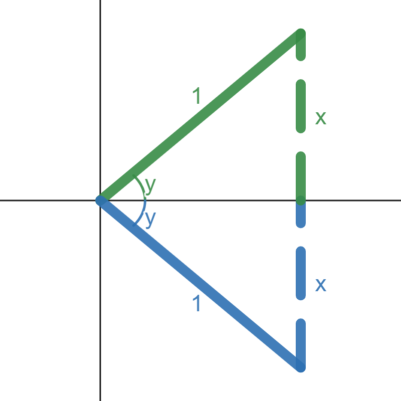
Figure \(\PageIndex{2}\): A graph of where the arcsine returns and the corresponding triangles.

From Figure \(\PageIndex{2}\), we can see that the length of the adjacent side, in either case, is \(+\sqrt{1 - x^2}\) (positive because these triangles both share adjacent sides along the positive \(x\)-axis).

If \(\sin{(y)} = x\), then

\[ \begin{array}{rclcrcl}
\dfrac{d}{dx}\left( \sin{(y)} \right) & = & \dfrac{d}{dx}(x) & \implies & \cos{(y)} \dfrac{dy}{dx} & = & 1 \\
& & & \implies & \dfrac{dy}{dx} & = & \dfrac{1}{\cos{(y)}} \\
& & & \implies & & = & \dfrac{1}{\sqrt{1 - x^2}}. \\
\end{array} \nonumber \]

Q.E.D.

Caution

As was mentioned in chapter 1 of this textbook, the definition we use for the ranges of the secant and cosecant functions are very specific to this book. A lot of other texts use a different definition. I have chosen to restrict the ranges of the inverse cosecant to \((0,\pi/2] \cup (\pi,3\pi/2]\) and the inverse secant to \([0,\pi/2) \cup [\pi,3\pi/2)\).

This choice is made to avoid challenging issues in Calculus.

The proof we just did is indicative of the thought process you must go through when proving the derivative of an inverse trigonometric function. You must address the fact that the inverse function has a restricted range. The possible angles returned by an inverse trigonometric function are always limited to two quadrants, and for each such quadrant it is immensely helpful to draw a right triangle whose hypotenuse lies on the terminal side of an angle in that restricted quadrant.

Example \(\PageIndex{4}\): Finding the Derivative of an Inverse Trigonometric Function

Find the derivative of \(h(x)=\sin^{−1}(2x^3).\)

Solution

\[ \begin{array}{rcl}
\dfrac{d}{dx} \left( \sin^{-1}{(2x^3)} \right) & = & \dfrac{1}{\sqrt{1 - \left(2x^3\right)^2}} \cdot \dfrac{d}{dx}\left( 2x^3\right) \\
 & = & \dfrac{1}{\sqrt{1 - 4x^6}} \cdot 6x^2 \\
 & = & \dfrac{6x^2}{\sqrt{1 - 4x^6}} \\
\end{array} \nonumber \]

Exercise \(\PageIndex{4}\)

Use the inverse function theorem to find the derivative of \(g(x)=\tan^{−1}x\).

Hint

The inverse of \(g(x)\) is \(f(x)=\tan x\). Use Example \(\PageIndex{4A}\) as a guide.

Answer

\(g^{\prime}(x)=\frac{1}{1+x^2}\)

Example \(\PageIndex{5}\): Applying Differentiation Formulas to an Inverse Tangent Function

Find the derivative of \(f(x)=\tan^{−1}(x^2).\)

Solution

\[ \begin{array}{rcl}
\dfrac{d}{dx} \left( \tan^{-1}{(x^2)} \right) & = & \dfrac{1}{1 + \left( x^2 \right)^2 } \cdot \dfrac{d}{dx} \left( x^2 \right) \\
 & = & \dfrac{2x}{1 + x^4} \\
\end{array} \nonumber \]

Example \(\PageIndex{6}\): Applying Differentiation Formulas to an Inverse Cosecant Function

Find the derivative of \(h(x)=x^2 \csc^{−1}{(x)}.\)

Solution

\[ \begin{array}{rcl}
\dfrac{d}{dx} \left( x^2 \csc^{-1}{(x)} \right) & = & 2x \csc^{-1}{(x)} - \dfrac{x^2}{x \sqrt{x^2 - 1}} \\
 & = & 2x \csc^{-1}{(x)} - \dfrac{x}{\sqrt{x^2 - 1}} \\
\end{array} \nonumber \]

Exercise \(\PageIndex{6}\)

Find the derivative of \(h(x)=\cos^{−1}(3x−1).\)

Answer

\(h^{\prime}(x)=\frac{−3}{\sqrt{6x−9x^2}}\)

Example \(\PageIndex{7}\): Applying the Inverse Tangent Function

The position of a particle at time \(t\) is given by \(s(t)=\tan^{−1}\left(\frac{1}{t}\right)\) for \(t \geq \ce{1/2}\). Find the velocity of the particle at time \( t=1\).

Solution

Begin by differentiating \(s(t)\) in order to find \(v(t)\).Thus,

\[v(t)=s^{\prime}(t)=\dfrac{1}{1+\left(\frac{1}{t}\right)^2} \cdot \dfrac{−1}{t^2}.\nonumber\]

Simplifying, we have

\[v(t)=−\dfrac{1}{t^2+1}.\nonumber\]

Thus, \(v(1)=−\frac{1}{2}.\)

Exercise \(\PageIndex{7}\)

Find the equation of the line tangent to the graph of \(f(x)=\sin^{−1}x\) at \(x=0.\)

Hint

\(f^{\prime}(0)\) is the slope of the tangent line.

Answer

\(y=x\)

Derivatives of Inverse Hyperbolic Functions

Looking at the graphs of the hyperbolic functions, we see that with appropriate range restrictions, they all have inverses. Most of the necessary range restrictions can be discerned by close examination of the graphs. The domains and ranges of the inverse hyperbolic functions are summarized in Table \(\PageIndex{1}\).

Table \(\PageIndex{1}\): Domains and Ranges of the Inverse Hyperbolic Functions

Function	Domain	Range
\(\sinh^{−1}x\)	\( (−\infty, \infty) \)	\( (− \infty, \infty) \)
\(\cosh^{−1}x\)	\( (1, \infty) \)	\( [0, \infty) \)
\(\tanh^{−1}x\)	\( (−1,1) \)	\( (− \infty, \infty) \)
\(\coth^{−1}x\)	\( (− \infty,1)∪(1, \infty) \)	\( (− \infty,0)∪(0, \infty) \)
\(\text{sech}^{−1}x\)	\( (0,1) \)	\( [0, \infty) \)
\(\text{csch}^{−1}x\)	\( (− \infty,0)∪(0, \infty) \)	\( (− \infty,0)∪(0, \infty) \)

The graphs of the inverse hyperbolic functions are shown in the following figure.

Figure \(\PageIndex{3}\): Graphs of the inverse hyperbolic functions.

To find the derivatives of the inverse functions, we use implicit differentiation. We have

\[ \begin{array}{rcl}
y & = & \sinh^{−1}x \\
\sinh y &= & x \\
\dfrac{d}{dx} \sinh y & = & \dfrac{d}{dx}x \\
\cosh y\dfrac{dy}{dx} & = & 1. \\
\end{array} \nonumber \]

Recall that \(\cosh^2y−\sinh^2y=1,\) so \(\cosh y=\sqrt{1+\sinh^2y}\).Then,

\[\dfrac{dy}{dx}=\dfrac{1}{\cosh y}=\dfrac{1}{\sqrt{1+\sinh^2y}}=\dfrac{1}{\sqrt{1+x^2}}. \nonumber \]

We can derive differentiation formulas for the other inverse hyperbolic functions in a similar fashion. These differentiation formulas are summarized in Table \(\PageIndex{2}\).

Table \(\PageIndex{2}\): Derivatives of the Inverse Hyperbolic Functions

\(f(x)\)	\(\dfrac{d}{dx}f(x)\)
\(\sinh^{−1}x\)	\(\dfrac{1}{\sqrt{1+x^2}}\)
\(\cosh^{−1}x\)	\(\dfrac{1}{\sqrt{x^2−1}}\)
\(\tanh^{−1}x\)	\(\dfrac{1}{1−x^2}\)
\(\coth^{−1}x\)	\(\dfrac{1}{1−x^2}\)
\(\text{sech}^{−1}x\)	\(\dfrac{−1}{x\sqrt{1−x^2}}\)
\(\text{csch}^{−1}x\)	\(\dfrac{−1}{|x|\sqrt{1+x^2}}\)

Note that the derivatives of \(\tanh^{−1}x\) and \(\coth^{−1}x\) are the same.

Example \(\PageIndex{8}\): Differentiating Inverse Hyperbolic Functions

Evaluate the following derivatives:

1. \(\frac{d}{dx}\left(\sinh^{−1}\left(\frac{x}{3}\right)\right)\)
2. \(\frac{d}{dx}\left(\tanh^{−1}x\right)^2\)

Solution

Using the formulas in Table \(\PageIndex{3}\) and the Chain Rule, we obtain the following results:

1. \(\frac{d}{dx}(\sinh^{−1}(\frac{x}{3}))=\frac{1}{3\sqrt{1+\frac{x^2}{9}}}=\frac{1}{\sqrt{9+x^2}}\)
2. \(\frac{d}{dx}(\tanh^{−1}x)^2=\frac{2(\tanh^{−1}x)}{1−x^2}\)

Exercise \(\PageIndex{8}\)

Evaluate the following derivatives:

1. \(\frac{d}{dx}(\cosh^{−1}(3x))\)
2. \(\frac{d}{dx}(\coth^{−1}x)^3\)

Hint

Use the formulas in Table \(\PageIndex{2}\) and apply the Chain Rule as necessary.

Answer a

\(\frac{d}{dx}(\cosh^{−1}(3x))=\frac{3}{\sqrt{9x^2−1}} \)

Answer b

\(\frac{d}{dx}(\coth^{−1}x)^3=\frac{3(\coth^{−1}x)^2}{1−x^2} \)

Key Concepts

• The inverse function theorem allows us to compute derivatives of inverse functions without using the limit definition of the derivative.
• We can use the inverse function theorem to develop differentiation formulas for the inverse trigonometric functions.

Key Equations

• Power Rule with rational exponents

\(\dfrac{d}{dx}\big(x^{m/n}\big)=\dfrac{m}{n}x^{(m/n)−1}.\)

• Derivative of inverse sine function

\(\dfrac{d}{dx}\big(\sin^{−1}x\big)=\dfrac{1}{\sqrt{1−x^2}}\)

• Derivative of inverse cosine function

\(\dfrac{d}{dx}\big(\cos^{−1}x\big)=\dfrac{−1}{\sqrt{1−x^2}}\)

Derivative of inverse tangent function

\(\dfrac{d}{dx}\big(\tan^{−1}x\big)=\dfrac{1}{1+x^2}\)

Derivative of inverse cotangent function

\(\dfrac{d}{dx}\big(\cot^{−1}x\big)=\dfrac{−1}{1+x^2}\)

Derivative of inverse secant function

\(\dfrac{d}{dx}\big(\sec^{−1}x\big)=\dfrac{1}{x\sqrt{x^2−1}}\)

Derivative of inverse cosecant function

\(\dfrac{d}{dx}\big(\csc^{−1}x\big)=\dfrac{−1}{x\sqrt{x^2−1}}\)

Contributors and Attributions

• Gilbert Strang (MIT) and Edwin “Jed” Herman (Harvey Mudd) with many contributing authors. This content by OpenStax is licensed with a CC-BY-SA-NC 4.0 license. Download for free at http://cnx.org.

• Paul Seeburger (Monroe Community College) added the second half of Example \(\PageIndex{2}\).