3.2: The Mean Value Theorem

Learning Objectives Explain the meaning of Rolle's theorem Describe the significance of the Mean Value Theorem Use the Racetrack Principle to prove inequalities State two critical consequences of the Mean Value Theorem

Hawk A.I. Section-Specific Tutor Please note that, to access the Hawk A.I. Tutor, you will need a (free) OpenAI account.

The Mean Value Theorem is one of the most important theorems in Calculus. We look at some of its implications at the end of this section. First, let's start with a particular case of the Mean Value Theorem, called Rolle's Theorem.

Rolle’s Theorem

Informally, Rolle's Theorem states that if the outputs of a differentiable function \(f\) are equal at the endpoints of an interval, then there must be an interior point \(c\) where \(f^{\prime}(c)=0\). Figure \(\PageIndex{1}\) illustrates this theorem.

Figure \(\PageIndex{1}\): If a differentiable function \(f\) satisfies \(f(a)=f(b)\), then its derivative must be zero at some point(s) between \(a\) and \(b\).

Theorem: Rolle's Theorem

Let \(f\) be a continuous function over the closed interval \([a,b]\) and differentiable over the open interval \((a,b)\) such that \(f(a)=f(b)\). There then exists at least one \(c \in (a,b)\) such that \(f^{\prime}(c)=0\).

Proof

Let \(k=f(a)=f(b)\). We consider three cases:

Case 1 - \(f(x)=k\) for all \(x \in (a,b)\): If \(f(x)=k\) for all \(x \in (a,b)\), then \(f^{\prime}(x)=0\) for all \(x \in (a,b)\).

Case 2 - There exists \(x \in (a,b)\) such that \(f(x)>k\): Since \(f\) is a continuous function over the closed, bounded interval \([a,b]\), by the Extreme Value Theorem, it has an absolute maximum. Also, since there is a point \(x \in (a,b)\) such that \(f(x)>k\), the absolute maximum is greater than \(k\). Therefore, the absolute maximum does not occur at either endpoint. As a result, the absolute maximum must occur at an interior point \(c \in (a,b)\). Because \(f\) has a maximum at an interior point \(c\), and \(f\) is differentiable at \(c\), by Fermat’s Theorem, \(f^{\prime}(c)=0\).

Case 3 - There exists \(x \in (a,b)\) such that \(f(x)<k\): The case when there exists a point \(x \in (a,b)\) such that \(f(x)<k\) is analogous to case 2, with maximum replaced by minimum.

Q.E.D.

Caution: \( f \) Must Be Differentiable!

An important point about Rolle's Theorem is that the differentiability of the function \(f\) is critical. If \(f\) is not differentiable, even at a single point, the result may not hold. For example, the function \(f(x)=|x|−1\) is continuous over the closed interval \([−1,1]\) and \(f(−1)=0=f(1)\), but \(f^{\prime}(c) \neq 0\) for any \(c \in (−1,1)\) as shown Figure \( \PageIndex{ 2 } \).

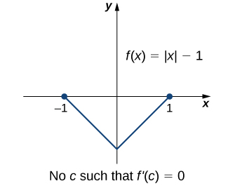
Figure \(\PageIndex{2}\): Since \(f(x)=|x|−1\) is not differentiable at \(x=0\), the conditions of Rolle's Theorem are not satisfied. In fact, the conclusion does not hold here; there is no \(c \in (−1,1)\) such that \(f^{\prime}(c)=0\).

Let's now consider functions that satisfy the conditions of Rolle's Theorem and calculate explicitly the numbers \(c\) where \(f^{\prime}(c)=0\).

Example \(\PageIndex{1}\)

For each of the following functions, verify that the function satisfies the criteria stated in Rolle's Theorem and find all numbers \(c\) in the given interval where \(f^{\prime}(c)=0\).

1. \(f(x)=x^2+2x\) over \([−2,0]\)
2. \(f(x)=x^3−4x\) over \([−2,2]\)

Solutions

1. Since \(f\) is a polynomial, it is continuous and differentiable everywhere. In addition, \(f(−2)=0=f(0)\). Therefore, \(f\) satisfies the criteria of Rolle's Theorem. We conclude that there exists at least one value \(c \in (−2,0)\) such that \(f^{\prime}(c)=0\). Since \(f^{\prime}(x)=2x+2=2(x+1)\), we see that \(f^{\prime}(c)=2(c+1)=0\) implies \(c=−1\) as shown in Figure \( \PageIndex{ 3 } \).

   
   Figure \(\PageIndex{3}\): This function is continuous and differentiable over \([−2,0]\), \(f^{\prime}(c)=0\) when \(c=−1\).

2. As in part a., \(f\) is a polynomial and is continuous and differentiable everywhere. Also, \(f(−2)=0=f(2)\). That said, \(f\) satisfies the criteria of Rolle's Theorem. Differentiating, we find that \(f^{\prime}(x)=3x^2−4\). Therefore, \(f^{\prime}(c)=0\) when \(x= \pm \frac{2}{\sqrt{3}}\). Both points are in the interval \([−2,2]\), and, therefore, both points satisfy the conclusion of Rolle's Theorem as shown in Figure \( \PageIndex{ 4 } \).

   
   Figure \(\PageIndex{4}\): For this polynomial over \([−2,2], f^{\prime}(c)=0\) at \(x= \pm 2/\sqrt{3}\).

Checkpoint \(\PageIndex{1}\)

Verify that the function \(f(x)=2x^2−8x+6\) defined over the interval \([1,3]\) satisfies the conditions of Rolle’s Theorem. Find all numbers \(c\) guaranteed by Rolle’s Theorem.

Answer

\(c=2\)

A creative use of Rolle's Theorem is to prove a given equation has exactly one root. We did something almost like this when working through continuity in the limits unit. Recall, by the Intermediate Value Theorem, if \( f \) is a continuous function on a closed interval \([a,b]\), where the signs of \(f(a)\) and \(f(b)\) are opposite, there must exist some number \(c \in (a,b)\) such that \(f(c) = 0\). This was used to show the existence of a root to a given equation in the interval \([a,b]\). This proof is commonly called an existence proof because you are proving something (a root) exists.

We are now extending this concept to a uniqueness proof. We not only want to prove that there exists a root to a given equation, but we also want to prove that root is the only such root (i.e., that the root is unique).

Example \(\PageIndex{2}\)

Prove the equation \(2 x = \cos{(x)}\) has only one solution.

Solution

Existence. We begin our proof by showing that a solution to the equation exists.

Let \(f(x) = 2x - \cos{(x)}\). Then \(f\) has a zero precisely when \(2 x = \cos{(x)}\) has a solution. Since \(f\) is the sum of a polynomial function and a cosine function, both of which are continuous on \(\mathbb{R}\), \(f\) is continuous on \(\mathbb{R}\). Moreover, \(f(0) = -1 \lt 0\) and \(f(\pi/2) = \pi \gt 0\). By the Intermediate Value Theorem, \(f\) must have a zero on the interval \((0, \pi/2)\). Therefore, the given equation must have a solution on the interval \( (0, \pi/2) \).

Uniqueness. We continue our proof by showing that the solution on the interval \( (0, \pi/2) \) must be the only solution. To showcase this result, we argue using a proof by contradiction.¹

Let's assume that the given equation has more than one solution. This means the function, \( f \), would have more than one zero. That is, there must exist two values, \( c \) and \( d \), such that \( f(c) = 0 = f(d) \), where \( c \neq d \).

We have the following three conditions met:

1. \( f \) is continuous on the closed interval \( [c,d] \),
2. \( f^{\prime}(x) = 2 + \sin{(x)} \) exists on the open interval \( (c,d) \), and
3. \( f(c) = f(d). \)

Thus, by Rolle's Theorem, there must exist a number \( k \in (c,d) \) such that \( f^{\prime}(k) = 0. \)

However, \( f^{\prime}(x) = 2 + \sin{(x)} \ge 1 \) for all \( x \in \mathbb{R} \). This contradicts the statement that \( f^{\prime}(k) = 0 \) for some \( k \in (c,d) \). Hence, our only assumption, that the given equation has more than one solution, must be incorrect. Since we have already shown that a solution exists, the equation must only have that one solution.

Q.E.D.

The Mean Value Theorem and Its Meaning

Rolle’s Theorem is a special case of the Mean Value Theorem. In Rolle's Theorem, we consider differentiable functions on closed intervals having the same function values at the endpoints of the interval. The Mean Value Theorem generalizes Rolle's Theorem by considering functions that do not necessarily have the same function values at the endpoints. Consequently, we can view the Mean Value Theorem as a slanted version of Rolle's Theorem (see Figure \(\PageIndex{5}\)). The Mean Value Theorem states that if \(f\) is continuous over the closed interval \([a,b]\) and differentiable over the open interval \((a,b)\), then there exists a point \(c \in (a,b)\) such that the tangent line to the graph of \(f\) at \(c\) is parallel to the secant line connecting \((a,f(a))\) and \((b,f(b))\).

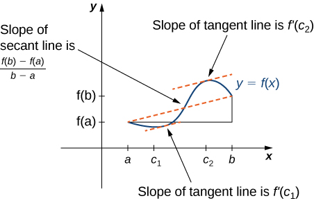
Figure \( \PageIndex{5} \): The Mean Value Theorem says that for a function that meets its conditions, at some point, the tangent line has the same slope as the secant line between the ends. For this function, there are two values \(c_1\) and \(c_2\) such that the tangent line to \(f\) at \(c_1\) and \(c_2\) has the same slope as the secant line.

Theorem: The Mean Value Theorem (MVT)

Let \(f\) be continuous over the closed interval \([a,b]\) and differentiable over the open interval \((a,b)\). Then, there exists at least one point \(c \in (a,b)\) such that\[f^{\prime}(c)=\dfrac{f(b)−f(a)}{b−a} \nonumber \]

Proof

The proof follows from Rolle's Theorem by introducing an appropriate function that satisfies the criteria of Rolle's Theorem. Consider the line connecting \((a,f(a))\) and \((b,f(b))\). Since the slope of that line is\[\dfrac{f(b)−f(a)}{b−a} \nonumber \]and the line passes through the point \((a,f(a))\), the equation of that line can be written as\[y=\dfrac{f(b)−f(a)}{b−a}(x−a)+f(a). \nonumber \]Let \(g(x)\) denote the vertical difference between the point \((x,f(x))\) and the point \((x,y)\) on that line. Therefore,\[g(x)=f(x)−\left[\dfrac{f(b)−f(a)}{b−a}(x−a)+f(a)\right]. \nonumber \]

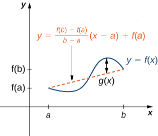
Figure \(\PageIndex{6}\): The value \(g(x)\) is the vertical difference between the point \((x,f(x))\) and the point \((x,y)\) on the secant line connecting \((a,f(a))\) and \((b,f(b))\).

Since the graph of \(f\) intersects the secant line when \(x=a\) and \(x=b\), we see that \(g(a)=0=g(b)\). Since \(f\) is a differentiable function over \((a,b)\), \(g\) is also a differentiable function over \((a,b)\). Furthermore, since \(f\) is continuous over \([a,b]\), \(g\) is also continuous over \([a,b]\). Therefore, \(g\) satisfies the criteria of Rolle's Theorem. Consequently, there exists a point \(c \in (a,b)\) such that \(g^{\prime}(c)=0\). Since\[g^{\prime}(x)=f^{\prime}(x)−\dfrac{f(b)−f(a)}{b−a}, \nonumber \]we see that\[g^{\prime}(c)=f^{\prime}(c)−\dfrac{f(b)−f(a)}{b−a}. \nonumber \]Since \(g^{\prime}(c)=0\), we conclude that\[f^{\prime}(c)=\dfrac{f(b)−f(a)}{b−a}. \nonumber \]

Q.E.D.

As a notational point, the Mean Value Theorem is often written as the MVT. In the following example, we show how the MVT can be applied to the function \(f(x)=\sqrt{x}\) over the interval \([0,9]\). The method is the same for other functions, although sometimes with more interesting consequences.

Example \(\PageIndex{3}\)

For \(f(x)=\sqrt{x}\) over the interval \([0,9]\), show that \(f\) satisfies the hypothesis of the Mean Value Theorem. Find the numbers \(c\) guaranteed by the Mean Value Theorem.

Solution

We know that \(f(x)=\sqrt{x}\) is continuous over \([0,9]\) and differentiable over \((0,9)\). Therefore, \(f\) satisfies the hypotheses of the Mean Value Theorem. As such, there must exist at least one value \(c \in (0,9)\) such that \(f^{\prime}(c)\) is equal to the slope of the line connecting \((0,f(0))\) and \((9,f(9))\) (see Figure \(\PageIndex{7}\)). To determine the value(s) of \(c\), first calculate the derivative of \(f\).\[f^{\prime}(x)=\dfrac{1}{(2\sqrt{x})}.\nonumber \]The slope of the line connecting \((0,f(0))\) and \((9,f(9))\) is given by\[\dfrac{f(9)−f(0)}{9−0}=\dfrac{\sqrt{9}−\sqrt{0}}{9−0}=\dfrac{3}{9}=\dfrac{1}{3}. \nonumber \]We want to find \(c\) such that \(f^{\prime}(c)=\frac{1}{3}\). That is, we want to find \(c\) such that\[\dfrac{1}{2\sqrt{c}}=\dfrac{1}{3}. \nonumber \]Solving this equation for \(c\), we obtain \(c=\frac{9}{4}\). At this point, the slope of the tangent line equals the slope of the line joining the endpoints.

Figure \(\PageIndex{7}\): The slope of the tangent line at \(c=9/4\) is the same as the slope of the line segment connecting (0,0) and (9,3).

One application that helps illustrate the Mean Value Theorem involves velocity. For example, suppose we drive a car for one hour down a straight road with an average velocity of 45 miles per hour. Let \(s(t)\) and \(v(t)\) denote the position and velocity of the car, respectively, for \(0 \leq t \leq 1\) hour. Assuming that the position function, \(s(t)\), is differentiable, we can apply the Mean Value Theorem to conclude that, at some time \(c \in (0,1)\), the speed of the car was precisely \[v(c)=s^{\prime}(c)=\dfrac{s(1)−s(0)}{1−0}=45\,\text{mph.} \nonumber \]

Example \(\PageIndex{4}\)

If a rock is dropped from a height of 100 ft, its position \(t\) seconds after it is dropped until it hits the ground is given by the function \(s(t)=−16t^2+100\).

1. Determine how long it takes before the rock hits the ground.
2. Find the average velocity \(v_{avg}\) of the rock for when the rock is released and the rock hits the ground.
3. Find the time \(t\) guaranteed by the Mean Value Theorem when the instantaneous velocity of the rock is \(v_{avg}\).

Solutions

1. When the rock hits the ground, its position is \(s(t)=0\). Solving the equation \(−16t^2+100=0\) for \(t\), we find that \(t= \pm \frac{5}{2}\) seconds. Since we are only considering \(t \geq 0\), the ball will hit the ground \(\frac{5}{2}\) seconds after it is dropped.
2. The average velocity is given by\[v_{avg}=\dfrac{s(5/2)−s(0)}{5/2−0}=\dfrac{0−100}{5/2}=−40\,\text{ft/sec}. \nonumber \]
3. The instantaneous velocity is given by the derivative of the position function. Therefore, we need to find a time \(t\) such that \(v(t)=s^{\prime}(t)=v_{avg}=−40\) feet per second. Since \(s(t)\) is continuous over the interval \(\left[0,\frac{5}{2}\right]\) and differentiable over the interval \(\left(0,\frac{5}{2}\right)\), by the Mean Value Theorem, there is guaranteed to be a point \(c \in \left(0,\frac{5}{2}\right)\) such that\[s^{\prime}(c)=\dfrac{s(5/2)−s(0)}{5/2−0}=−40. \nonumber \]Taking the derivative of the position function \(s(t)\), we find that \(s^{\prime}(t)=−32t\). Therefore, the equation reduces to \(s^{\prime}(c)=−32c=−40\). Solving this equation for \(c\), we have \(c=\frac{5}{4}\). Therefore, \(\frac{5}{4}\) seconds after the rock is dropped, the instantaneous velocity equals the average velocity of the rock during its free fall: \(−40\) feet per second.

   
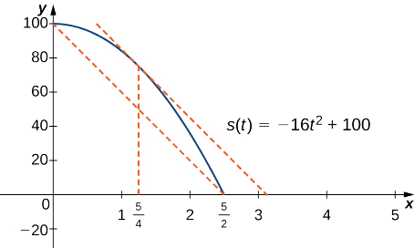
   Figure \(\PageIndex{8}\): At time \(t=5/4\) sec, the velocity of the rock is equal to its average velocity from the time it is dropped until it hits the ground.

Checkpoint \(\PageIndex{4}\)

Suppose a ball is dropped from a height of 200 ft. Its position at time \(t\) is \(s(t)=−16t^2+200\). Find the time \(t\) when the instantaneous velocity of the ball equals its average velocity.

Answer

\(\frac{5}{2\sqrt{2}}\) seconds

Corollaries of the Mean Value Theorem

Let's look at three Mean Value Theorem corollaries. These results have important consequences, which we will use in upcoming sections.

At this point, we know the derivative is zero if we are given a constant function. The Mean Value Theorem allows us to conclude that the converse is also true. In particular, if \(f^{\prime}(x)=0\) for all \(x\) in some interval \(I\), then \(f(x)\) is constant over that interval. This result may seem intuitively obvious, but it has important implications that are not obvious, and we discuss them shortly.

Corollary: Functions with a Derivative of Zero

Let \(f\) be differentiable over an interval \(I\). If \(f^{\prime}(x)=0\) for all \(x \in I\), then \(f(x)=\) constant for all \(x \in I\).

Proof

Since \(f\) is differentiable over \(I\), \(f\) must be continuous over \(I\). Suppose \(f(x)\) is not constant for all \(x\) in \(I\). Then there exist \(a,b \in I\), where \(a \neq b\) and \(f(a) \neq f(b)\). Choose the notation so that \(a<b\). Therefore,\[\dfrac{f(b)−f(a)}{b−a} \neq 0. \nonumber \]Since \(f\) is a differentiable function, by the Mean Value Theorem, there exists \(c \in (a,b)\) such that\[f^{\prime}(c)=\dfrac{f(b)−f(a)}{b−a}. \nonumber \]Therefore, there exists \(c \in I\) such that \(f^{\prime}(c) \neq 0\), which contradicts the assumption that \(f^{\prime}(x)=0\) for all \(x \in I\).

Q.E.D.

From this corollary, it follows that if two functions have the same derivative, they differ by, at most, a constant.

Corollary: Constant Difference Theorem

If \(f\) and \(g\) are differentiable over an interval \(I\) and \(f^{\prime}(x)=g^{\prime}(x)\) for all \(x \in I\), then \(f(x)=g(x)+C\) for some constant \(C\).

Proof

Let \(h(x)=f(x)−g(x)\). Then, \(h^{\prime}(x)=f^{\prime}(x)−g^{\prime}(x)=0\) for all \(x \in I\). By the previous corollary, there is a constant \(C\) such that \(h(x)=C\) for all \(x \in I\). Therefore, \(f(x)=g(x)+C\) for all \(x \in I\).

Q.E.D.

This corollary can be used to prove identities (like your trigonometric identities from your previous Trigonometry course).

Example \(\PageIndex{5}\)

Prove the following identity.\[ 2 \sin^{-1}{(x)} = \cos^{-1}{(1 - 2x^2)}, \text{ where }x \geq 0 \nonumber \]

Solution

Let \( f(x) = 2 \sin^{-1}{(x)} \) and \( g(x) = \cos^{-1}{(1 - 2x^2)} \). Note that the normal domain of \( f \) is \( [-1, 1] \) and we could quickly determine the domain of \( g \) to also be \( [-1, 1] \); however, we have been told that \( x \geq 0 \). Therefore, the domains of both functions are \( [0, 1] \).

Computing the derivatives, we get\[ f^{\prime}(x) = 2 \cdot \dfrac{1}{\sqrt{1 - x^2}} = \dfrac{2}{\sqrt{1 - x^2}} \nonumber \]and\[ \begin{array}{rclcl}
g^{\prime}(x) & = & -\dfrac{1}{\sqrt{1 - \left(1 - 2x^2\right)^2}} \cdot \left(-4x\right) & & \\[6pt]
& = & \dfrac{4x}{\sqrt{1 - \left(1 - 4x^2 + 4x^4\right)}} & & \\[6pt]
& = & \dfrac{4x}{\sqrt{4x^2 - 4x^4}} & & \\[6pt]
& = & \dfrac{4x}{2 x \sqrt{1 - x^2}} & \quad & \left(\text{since }x \geq 0\right) \\[6pt]
& = & \dfrac{2}{\sqrt{1 - x^2}} & & \\[6pt]
& = & f^{\prime}(x) & & \\[6pt]
\end{array} \nonumber \]Since \( f^{\prime}(x) = g^{\prime}(x) \) for \( x \in (0,1) \), \( f(x) = g(x) + C \) for all \( x \in (0,1) \) by the Constant Difference Theorem. That is, there exists \( C \) such that\[ 2 \sin^{-1}{(x)} = \cos^{-1}{(1 - 2x^2)} + C \nonumber \]Since this equation is true for all \( x \in (0,1) \), we can let \( x \) be any value in \( (0,1) \) to find the value of \( C \). Let \( x = \frac{1}{2} \). Then\[ 2 \sin^{-1}{\left(\dfrac{1}{2}\right)} = \cos^{-1}{\left(1 - 2\left(\dfrac{1}{2}\right)^2 \right)} + C \implies 2 \left(\dfrac{\pi}{6}\right) = \cos^{-1}{\left(\dfrac{1}{2}\right)} + C \implies \dfrac{\pi}{3} = \dfrac{\pi}{3} + C \implies C = 0. \nonumber \]To check the edges of the domain, let \( x = 0 \) and \( x = 1 \) in the original equation to get \( 0 = 0 \) and \( \pi = \pi \), respectively. Thus, the identity is true for all \( x \in [0,1] \).

A final corollary adds a unique use of the Mean Value Theorem to our toolbox. In my undergraduate studies, I had moments when I required an inequality to be true but had no idea how to show it was true. For example, there might have been a moment when I needed the inequality\[ \ln{(x)} \leq x - 1, \text{ for }x \geq 1 \nonumber \]to be true, but I had no clue how to show the truthfulness of the statement. Many students would "hand-wave" the process and say, "This is true." However, at this level, that type of justification is insufficient. This is where the Racetrack Principle comes into play.

Corollary: The Racetrack Principle

If \( f \) and \( g \) are continuous for all \( x \geq a \) and differentiable for all \( x \gt a \), and if \( f(a) = g(a) \) and \( f^{\prime}(x) \ge g^{\prime}(x) \) for all \( x \gt a \), then \( f(x) \ge g(x) \) for all \( x \ge a \).

Proof

Let \( f \) and \( g \) be continuous functions on the interval \( [a, \infty) \), and suppose both are differentiable on \( (a, \infty) \). Also, suppose \( f(a) = g(a) \) and \( f^{\prime}(x) \ge g^{\prime}(x) \) for all \( x \gt a \).

Let \( h(x) = f(x) - g(x) \). Then \( h \) is continuous on \( [a,\infty) \) and differentiable on \( (a,\infty) \). Moreover, \( h(a) = f(a) - g(a) = 0 \) and \( h^{\prime}(x) = f^{\prime}(x) - g^{\prime}(x) \ge 0 \) for all \( x \gt a \).

If we let \( b \gt a \) be arbitrary, then by the MVT there exists \( c \in (a,b) \) such that\[ h^{\prime}(c) = \dfrac{h(b) - h(a)}{b - a}. \nonumber \]However, we know that \( h^{\prime}(c) \ge 0 \) (since \( c \gt a \)). Therefore,\[ h^{\prime}(c) = \dfrac{h(b) - h(a)}{b - a} \geq 0. \nonumber \]Since \( b \gt a \), we can multiply all three side of this inequality by \((b - a)\) without changing the inequality signs to get\[ h^{\prime}(c) (b - a) = h(b) - h(a) \geq 0. \nonumber \]This means that\[ \begin{array}{rclcl}
f(b) - g(b) - \left(f(a) - g(a)\right) & \geq & 0 & \quad & \left(\text{substituting }h(a) = f(a) - g(a)\right) \\[6pt]
f(b) - g(b) - \left(0\right) & \geq & 0 & \quad & \left(\text{using the assumption that }f(a) = g(a)\right) \\[6pt]
f(b) & \geq & g(b) & & \\[6pt]
\end{array} \nonumber \]Since \( b \) was arbitrary, \( f(x) \geq g(x) \) for all \( x \geq a \).

Q.E.D.

This is called the Racetrack Principle because you can imagine the validity of this statement if you visualize a racetrack with two cars. Their positions (the functions) are continuous and differentiable (at least for \( x \gt a \)). This means that no car can teleport and radically change its position between moments in time, and their velocities always exist. These two conditions also allow us to immediately use the MVT if needed. Additionally, \( f(a) = g(a) \) means that the two cars start the race at the same position. Finally, \( f^{\prime}(x) \ge g^{\prime}(x) \) means that car "\( f \)" is as fast or faster than car "\( g \)." It should then make sense that car "\( f \)" will always be in the lead (or at least neck-and-neck with car "\( g \)").

Let's do an example to see the power of the Racetrack Principle.

Example \(\PageIndex{6}\)

Prove the inequality.\[ \ln{(x)} \leq x - 1, \text{ for }x \geq 1 \nonumber \]

Solution

Let \( f(x) = x - 1 \) and \( g(x) = \ln{(x)} \). Both functions are continuous and differentiable for all \( x \gt 0 \). Thus, they are continuous on \( [1,\infty) \) and differentiable on \( (1,\infty) \). Moreover, \( f(1) = 0 = g(1) \). Finally,\[ f^{\prime}(x) = 1 \text{ and } g^{\prime}(x) = 1/x . \nonumber \]For \( x \geq 1 \), \( f^{\prime} \) is always 1, but \( g^{\prime} \) is at most 1. In fact, for \( x \gt 1 \), \( g^{\prime}(x) \lt 1 \). Hence, \( f^{\prime}(x) \geq g^{\prime}(x) \) for all \( x \geq 1 \). Therefore, \( f(x) \geq g(x) \) for all \( x \geq 1 \), by the Racetrack Principle. That is,\[ x-1 \geq \ln{(x)}, \text{ for } x \geq 1. \nonumber \]

---

Footnotes

¹ A proof by contradiction is a proof style where you allow the antecedent (the "if" part) to be true and assume the consequent (the "then" part) is false. You will eventually arrive at a logical contradiction using logical, deductive arguments. If your arguments up to that point were clean, flawless, deductive logic, then the only weakness would have to be the assumption that the consequent was false. Thus, the consequent must have been true all along. This proof style is commonly used in courtrooms.