4.5: Graphing Using Calculus - Putting it Altogether

Learning Objectives

• Estimate the end behavior of a function as \(x\) increases or decreases without bound.
• Prove the equation of the slant asymptote to a function.
• Recognize an oblique asymptote on the graph of a function.
• Use the Guidelines to Graphing Using Calculus to analyze a function and its derivatives to accurately draw its graph.

We have gathered almost everything we need to accurately graph a given function using calculus. In this section, we finalize the topic by focusing on the end behavior of the graph of a function (specifically, whether or not the function has an oblique asymptote). Once that topic is finished, we present a tactic for graphing a function using calculus. 

End Behavior

The behavior of a function as \(x \to \pm \infty\) is called the function’s end behavior, and finding the end behavior of a function is the precise reason we introduced ourselves to l'Hospital's Rule. If \( f \) is a function of \( x \), then as \( x \to \infty \) or \( x \to -\infty \), the function could exhibit one of the following types of behavior:

1. No End Behavior: It can happen that a given function has a restricted domain. For example, it might be defined on the closed interval \( [-1,10] \). In these cases, the function does not have an end behavior because it is not defined as \(x \to \pm \infty\).
2. Horizontal Asymptote(s): If\[ \displaystyle \lim_{x \to \pm \infty}{f(x)} = L, \nonumber \]where \( L \) is finite, the function approaches a horizontal asymptote \(y=L\) as \( x \to \infty \) or as \( x \to -\infty \) (or both).
3. Slant Asymptote(s): If\[ \displaystyle \lim_{x \to \pm \infty}{f(x)} = \pm \infty, \nonumber \]then there is a little more work we need to do to determine if the function is mimicking a linear function near the edges of the domain.
4. Oscillatory Behavior: If \[ \displaystyle \lim_{x \to \pm \infty}{f(x)} \text{ DNE and is not }\pm \infty, \nonumber \]then the function does not have any asymptotic end behavior; however, it could be the case that the function is periodic and is following an oscillatory pattern as its end behavior.

Notes

• Each of the limits mentioned in the list above could have different asymptotes at each end of the function. That is, it's possible that \( \displaystyle \lim_{x \to -\infty}{f(x)} = 5 \) and \( \displaystyle \lim_{x \to \infty}{(f(x)} = -\infty \) (or a constant not equal to \(5\)). Do not assume that end behavior is symmetric.
• The list presented above is purposeful in its order.
  • When determining the end behavior of a given function, you immediately throw out the possibility for end behavior if your function has a restricted domain.
  • If the domain is unrestricted, then you take limits as \( x \to \pm \infty\).
    • If a limit is finite, then your function has a horizontal asymptote.
    • If the limit is infinite, then you have some extra work in determining if there is an underlying linear function the function is approaching as \(x \to \pm \infty\).
    • If the limit DNE and is not infinite, then your function might have oscillatory behavior and, if true, you will need to find the period of the oscillation.

Since we have already covered the topic of horizontal asymptotes (Chapter 2), the remainder of this subsection is dedicated to the discussion of slant asymptotes.

Definition: Slant Asymptote

The line \( y = mx + b \) is called a slant asymptote of the function \( f \) if

\[ \displaystyle \lim_{x \to \infty}{\left(f(x) - y\right)} = 0 \nonumber \]

or

\[ \displaystyle \lim_{x \to -\infty}{\left(f(x) - y\right)} = 0. \nonumber \]

Example \(\PageIndex{1}\)

Determine the slant asymptote of \( f(x) = 3x - 1 + e^{-2x} \)

Solution

As \( x \to \infty \), \( e^{-2x} \to 0 \) leaving us with \( 3x - 1 \). Thus, our claim is that \( y = 3x - 1 \) is a slant asymptote for the function \( f \) as \( x \to \infty \). To prove this statement, we use the definition.

\[ \begin{array}{rcl}
\displaystyle \lim_{x \to \infty} \left[ f(x) - y \right] & = & \displaystyle \lim_{x \to \infty}\left( 3x - 1 + e^{-2x} - (3x - 1) \right) \\
& = & \displaystyle \lim_{x \to \infty} e^{-2x} \\
& = & 0
\end{array} \nonumber \]

Thus, we have proven that \( y = 3x - 1 \) is a slant asymptote of \( f(x) = 3x - 1 + e^{-2x} \) as \( x \to \infty \).

It is important to mention here that the function in Example \( \PageIndex{1} \) does not have a slant asymptote as \( x \to -\infty \). This is because, as \( x \to -\infty \), there is not a term in \( f(x) \) that "disappears" to leave us with only a linear function.

Guidelines for Drawing the Graph of a Function

We now have enough analytical tools to draw graphs of a wide variety of algebraic and transcendental functions. Before showing how to graph specific functions, let’s look at a general strategy to use when graphing any function. Notice in the steps provided that I follow the Mathematical Mantra and step through the graphing process doing mathematics in the order we learned topics (with the exception of domain, which I often do first despite having learned that skill after learning how to find intercepts).

Tactic: Drawing the Graph of a Function

Given a function \(f\), use the following steps to sketch its graph by hand:

1. Domain: Determine the domain of the function.
2. Intercepts: Locate the \(x\)- and \(y\)-intercepts. Start creating a table of values to hold all of the data you are going to collect.
3. Symmetry: Determine if \(f\) is odd, even, or neither. If it's neither odd nor even, determine if it is periodic. This step is incredibly useful because once you know a function is, for example, odd, you can focus your energy on gathering all the information about the function for \( x \ge 0 \). After you precisely graph the function for these \(x\)-values, you can use the symmetry of the function to graph the other half.
4. Vertical Asymptotes: Use calculus to determine the behavior of the function near any vertical asymptote(s). This step will involve limits of the form\[ \displaystyle \lim_{x \to a^+}{f(x)} \text{ and } \displaystyle \lim_{x \to a^-}{f(x)}. \nonumber \]
5. End Behavior: Use calculus to determine the end behavior of the function. This step will involve limits of the form\[ \displaystyle \lim_{x \to \infty}{f(x)} \text{ and } \displaystyle \lim_{x \to −\infty}{f(x)}. \nonumber \]If either of these limits is a finite number \(L\), then \(y=L\) is a horizontal asymptote. If either of these limits is \(\infty\) or \(−\infty\), determine whether \(f\) has a slant asymptote.
6. First Derivative Information: Calculate \(f^{\prime}.\) Find all critical points and determine the intervals where \(f\) is increasing and where \(f\) is decreasing. Determine whether \(f\) has any local extrema.
7. Second Derivative Information: Calculate \(f^{\prime\prime}.\) Determine the intervals where \(f\) is concave up and where \(f\) is concave down. Use this information to determine whether \(f\) has any inflection points. The second derivative can also be used as an alternate means to determine or verify that \(f\) has a local extremum at a critical point.
8. Graph like a boss

Graphing Examples

Now let’s use this strategy to graph several different functions. We start by graphing a polynomial function.

Example \(\PageIndex{2}\)

Sketch a graph of \(R(x) = \frac{x^2}{x^2 + 1}.\)

Solution

Domain: Since \(R(x)\) is a rational function and its denominator, \( x^2 + 1 \), is always greater than or equal to \( 1 \), the domain is \( \mathbb{R} = (-\infty, \infty) \).

Intercepts: \( (0,0) \) is the only intercept.

Symmetry: \( R(-x) = \frac{(-x)^2}{(-x)^2 + 1} = \frac{x^2}{x^2 + 1} = R(x) \). Therefore, \( R \) is an even function. As such, we will limit the rest of our investigation to the interval \( [0, \infty) \) and reflect our graph across the \( y \)-axis when we are finished.

Vertical Asymptote(s): Since the domain of \( R \) is all real numbers and \( R \) is continuous, there is not going to be a vertical asymptote.

End Behavior: \[ \begin{array}{rcl}
\displaystyle \lim_{x \to \infty}{R(x)} & = & \displaystyle \lim_{x \to \infty}{ \dfrac{x^2}{x^2 + 1} } \\
 & = & \displaystyle \lim_{x \to \infty}{ \dfrac{1}{1 + \frac{1}{x^2}} } \\
 & = & \dfrac{1}{1 + 0} \\
 & = & 1  \\
\end{array} \nonumber \]Thus, \( R \) has a horizontal asymptote of \( y = 1 \) as \( x \to \infty \).

First Derivative Information: \[ \begin{array}{rcl}
R^{\prime}(x) & = & \dfrac{2x(x^2 + 1) - x^2(2x)}{(x^2 + 1)^2} \\
 & = & \dfrac{2x(x^2 + 1 - x^2)}{(x^2 + 1)^2} \\
 & = & \dfrac{2x}{(x^2 + 1)^2} \\
\end{array} \nonumber \]\( R^{\prime}(x) = 0 \), when \( x = 0 \). Otherwise, \( R^{\prime}(x) \) always exists. Thus, the only critical point of \( R \) is \( (0,0) \).

For \( x \gt 0 \), \( R^{\prime}(x) \gt 0 \). Therefore, \( R \) is increasing on the interval \( (0,\infty) \). Since \( R \) is an even function, \( R \) will be decreasing for \( x \lt 0 \). This means that \( (0,0) \) is a local minimum. All of the information can be seen on the number line for \( R^{\prime} \) in Figure \( \PageIndex{1}A \) below.

Figure \( \PageIndex{1}A \): The number line sign graph for \( R'^{\prime}\).

Second Derivative Information: \[ \begin{array}{rcl}
R^{\prime\prime}(x) & = & \dfrac{2(x^2 + 1)^2 - 2x \cdot 2(x^2 + 1) \cdot 2x)}{(x^2 + 1)^4} \\
 & = & \dfrac{(x^2 + 1)\left(2(x^2 + 1) - 8 x^2 \right)}{(x^2 + 1)^4} \\
 & = & \dfrac{-6x^2 + 2}{(x^2 + 1)^3} \\
 & = & \dfrac{-2(3 x^2 - 1)}{(x^2 + 1)^3} \\
\end{array} \nonumber \]\( R^{\prime\prime}(x) = 0 \), when \( x = \pm \frac{1}{\sqrt{3}} \). Otherwise, \( R^{\prime\prime}(x) \) always exists.

All of the information for \( R^{\prime\prime} \) can be seen on the number line for \( R^{\prime\prime} \) in Figure \( \PageIndex{1}B \) below (again, we only concern ourselves with \( x \)-values greater than \( 0 \) because \( R \) is even).

Figure \( \PageIndex{1}B \): The number line sign graph for \( R'^{\prime\prime}\).

Graph Like a Boss: Before graphing, it's best to collect all the important information into one clean "pile." It's also required that you compute the function values for \( R \) wherever there are local extrema, inflection points, and intercepts.

\( x \)	\( R(x) \)	Note(s)
\( 0 \)	\( 0 \)	\( x \)- and \( y \)-intercept, LMin
\( \dfrac{1}{\sqrt{3}} \approx 0.577 \)	\( \dfrac{1}{4} \)	I.P.

Symmetry: Even

Horizontal Asymptote: \( y = 1 \) as \( x \to \infty \)

Notice in Example \( \PageIndex{2} \) that we approximated the value of \( 1/\sqrt{3} \). When graphing by hand, it is sometimes necessary to use technology to get decimal approximations in order to properly place our points.

Example \(\PageIndex{3}\)

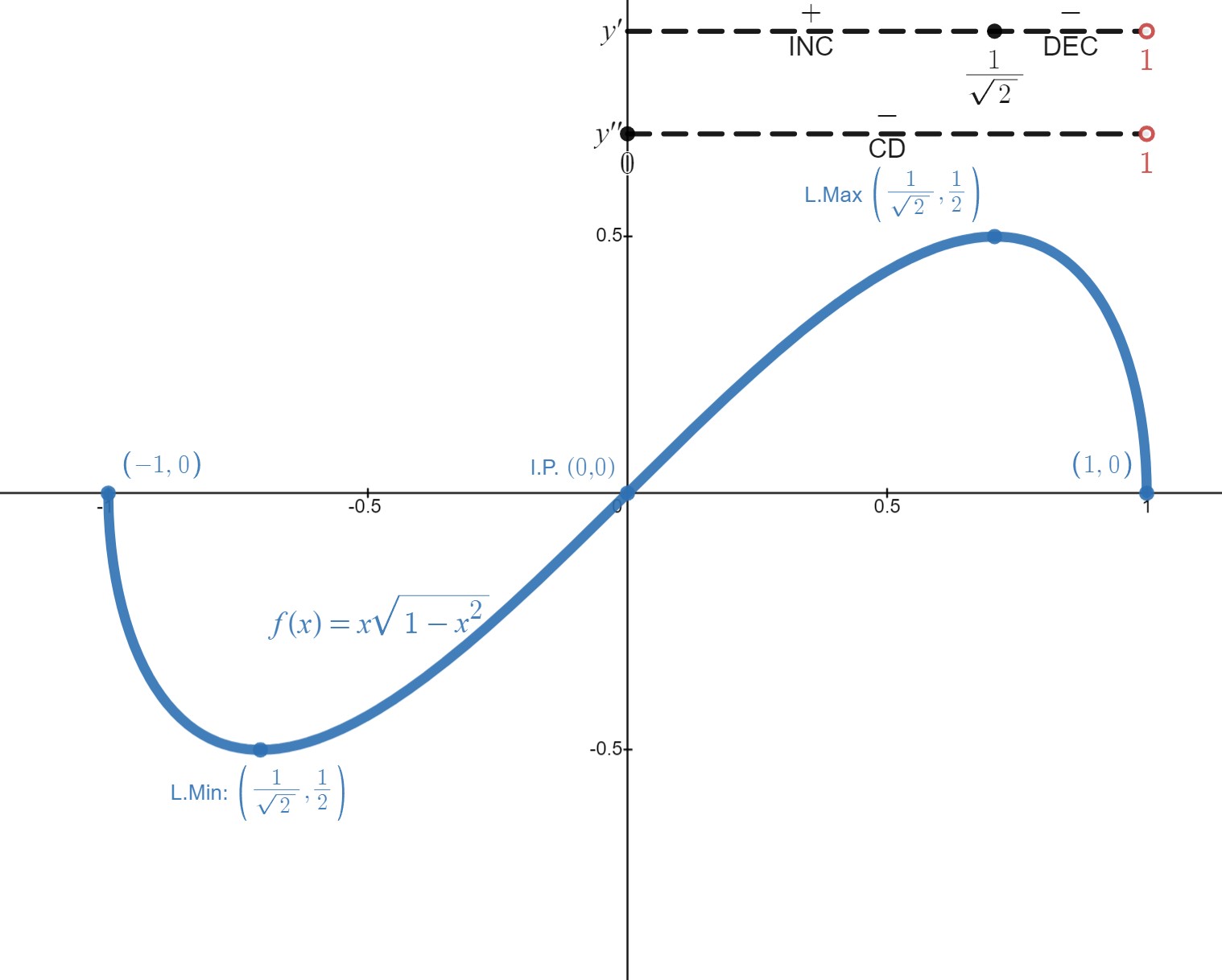
Sketch the graph of \(f(x) = x \sqrt{1 - x^2}\).

Solution

Domain: We require \( 1 - x^2 \ge 0 \implies 1 \ge x^2 \implies x \in [-1,1] \).

Intercepts: \( (0,0) \) and \( (\pm 1, 0) \) are the intercepts.

Symmetry: \( f(-x) = -x \sqrt{1 - (-x)^2} = -x \sqrt{1 - x^2} = -f(x) \). Therefore, \( f \) is an odd function. As such, we will limit the rest of our investigation to the interval \( [0, 1] \) and reflect our graph about the origin when we are finished.

Vertical Asymptote(s): Since the domain of \( f \) is a closed interval and \( f \) is continuous, there is not going to be a vertical asymptote.

End Behavior: Since the domain of \( f \) does not extend to infinity (in either direction), there is no end behavior to speak of.

First Derivative Information: \[ \begin{array}{rcl}
f^{\prime}(x) & = & \sqrt{1 - x^2} + x \cdot \dfrac{- 2 x}{2 \sqrt{1 - x^2}} \\
 & = & \sqrt{1 - x^2} - \dfrac{x^2}{\sqrt{1 - x^2}} \\
 & = & \dfrac{1 - x^2 - x^2}{\sqrt{1 - x^2}} \\
 & = & \dfrac{1 - 2 x^2}{\sqrt{1 - x^2}} \\
\end{array} \nonumber \]\( f^{\prime}(x) = 0 \), when \( x = \pm \frac{1}{\sqrt{2}} \), and \( f^{\prime}(x) \) does not exist at \( x = \pm 1 \). Since \( f \) is odd, we will only worry about \( x = \frac{1}{\sqrt{2}} \) and \( x = 1 \). The corresponding critical points are \( (1,0) \) and \( \left( \frac{1}{\sqrt{2}}, \frac{1}{2} \right) \). We first draw the number line.

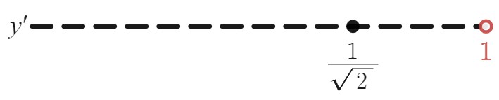
Testing each interval (and only substituting these values into the numerator of \( f^{\prime} \) because the denominator is always positive), we get \( f^{\prime}\left(\frac{1}{2}\right) \gt 0 \) and \( f^{\prime}\left( \frac{3}{4} \right) \lt 0 \). Therefore, \( f \) is increasing on \( \left( 0, \frac{1}{\sqrt{2}}\right) \) and decreasing on \( \left( \frac{1}{\sqrt{2}}, 0 \right) \). Hence, \( f \) has a local maximum at the point \( \left( \frac{1}{\sqrt{2}}, \frac{1}{2} \right) \). All of this information can be seen on the number line for \( f^{\prime} \) in Figure \( \PageIndex{2}A \) below.

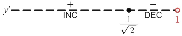
Figure \( \PageIndex{2}A \): The number line sign graph for \( f^{\prime} \).

Second Derivative Information: \[ \begin{array}{rcl}
f^{\prime\prime}(x) & = & \dfrac{-4x \sqrt{1 - x^2} - \left(1 - 2x^2 \right) \cdot \dfrac{-x}{\sqrt{1 - x^2}}}{1 - x^2} \\
 & = & \dfrac{-4x \left( 1 - x^2 \right) + x \left(1 - 2x^2 \right)}{\left(1 - x^2\right)^{3/2}} \\
 & = & \dfrac{x \left(2 x^2 - 3 \right)}{\left(1 - x^2\right)^{3/2}} \\
\end{array} \nonumber \]\( f^{\prime\prime}(x) = 0 \), when \( x = \pm \frac{\sqrt{6}}{2} \) and when \( x = 0 \). Moreover, \( f^{\prime\prime} \) does not exist when \( x = \pm 1 \). Again, since \( f \) is odd, we will only concern ourselves with \( x = 0 \), \( x = \frac{\sqrt{6}}{2} \), and \( x = 1 \); however, \( \frac{\sqrt{6}}{2} \gt 1 \) and, as such, is outside of the domain of \( f \). Hence, we only need worry about \( x = 0 \) and \( x = 1 \). Since \( f^{\prime\prime}\left( \frac{1}{2} \right) \lt 0 \), \( f \) is concave down on \( (0,1) \) (see Figure \( \PageIndex{2}B \)).

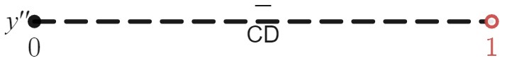
Figure \( \PageIndex{2}B \): The number line sign graph for \( f^{\prime\prime} \).

Graph Like a Boss:

\( x \)	\( R(x) \)	Note(s)
\( 0 \)	\( 0 \)	\( x \)- and \( y \)-intercept, I.P.
\( \dfrac{1}{\sqrt{2}} \approx 0.707 \)	\( \dfrac{1}{2} \)	L.Max
\( 1 \)	\( 0 \)	\( x \)-intercept

Symmetry: Odd

Note

Both functions in Examples \( \PageIndex{2} \) and \( \PageIndex{3} \) were continuous on their domains. Moreover, the domain of the function in Example \( \PageIndex{3} \) was a closed interval. When a function is continuous and has a domain of either \( \mathbb{R} \) or a closed interval, you can guarantee that the function does not have any vertical asymptotes. This is because of the definition of a vertical asymptote from Chapter 2. \( x = a \) is a vertical asymptote of \( f \) if any of the limits (single-sided or total) as \( x \to a \) becomes infinite. For a continuous function, this condition can only occur at the edge of its domain, and only if the domain doesn't include that edge.

Example \(\PageIndex{4}\)

Sketch the graph of \(f(x)=\frac{x^2}{x−1}\)

Solution

Domain: The domain of \(f\) is the set of all real numbers \(x\) except \(x=1.\)

Intercepts: We can see that when \(x=0, \,f(x)=0,\) so \((0,0)\) is the only intercept.

Symmetry: Since \( f(-x) = \frac{(-x)^2}{(-x) - 1} = \frac{x^2}{-x - 1} = - \frac{x^2}{x + 1} \neq \pm f(x) \), \( f \) is neither odd nor even.

Vertical Asymptote(s): To check for vertical asymptotes, look at where the denominator is zero. Here the denominator is zero at \(x=1.\) Looking at both one-sided limits as \(x \to 1,\) we find\[\displaystyle \lim_{x \to 1^+}\frac{x^2}{x−1}=\infty\nonumber\]and\[\displaystyle \lim_{x \to 1^−}\frac{x^2}{x−1}=−\infty.\nonumber\]Therefore, \(x=1\) is a vertical asymptote, and we have determined the behavior of \(f\) as \(x\) approaches \(1\) from the right and the left.

End Behavior: Evaluate the limits at infinity. Since the degree of the numerator is one more than the degree of the denominator, \(f\) must have a slant asymptote. To find the slant asymptote, use long division of polynomials to write\[f(x)=\dfrac{x^2}{x−1}=x+1+\dfrac{1}{x−1}.\nonumber\]Since \(\frac{1}{x−1} \to 0\) as \(x \to \pm \infty, f(x)\) approaches the line \(y=x+1\) as \(x \to \pm \infty\). The line \(y=x+1\) is a slant asymptote for \(f\).

First Derivative Information: Calculate the first derivative:\[f^{\prime}(x)=\dfrac{(x−1)(2x)−x^2(1)}{(x−1)^2}=\dfrac{x^2−2x}{(x−1)^2}.\nonumber\]We have \(f^{\prime}(x)=0\) when \(x^2−2x=x(x−2)=0\). Therefore, \(x=0\) and \(x=2\) are critical points. Since \(f\) is undefined at \(x=1\), we need to divide the interval \((−\infty,\infty)\) into the smaller intervals \((−\infty,0), (0,1), (1,2),\) and \((2,\infty)\), and choose a test point from each interval to evaluate the sign of \(f^{\prime}(x)\) in each of these smaller intervals. Doing so, we get the following sign chart for \( f^{\prime} \).

From this sign chart, we see that \(f\) has a local maximum at \(x=0\) and a local minimum at \(x=2\). The value of \(f\) at the local maximum is \(f(0)=0\) and the value of \(f\) at the local minimum is \(f(2)=4\). Therefore, \((0,0)\) and \((2,4)\) are important points on the graph.

Second Derivative Information: Calculate the second derivative:\[\begin{array}{rcl}
f^{\prime\prime}(x) & = & \dfrac{(x−1)^2(2x−2)−2(x−1)(x^2−2x)}{(x−1)^4} \\
& = & \dfrac{2(x−1)[(x−1)^2−(x^2−2x)]}{(x−1)^4}\\
& = & \dfrac{2[x^2-2x+1−x^2+2x]}{(x−1)^3}\\
& = & \dfrac{2}{(x−1)^3}. \\
\end{array}\nonumber\]We see that \(f^{\prime\prime}(x)\) is never zero or undefined for \(x\) in the domain of \(f\). Since \(f\) is undefined at \(x=1\), to check concavity we just divide the interval \((−\infty,\infty)\) into the two smaller intervals \((−\infty,1)\) and \((1,\infty)\), and choose a test point from each interval to evaluate the sign of \(f^{\prime\prime}(x)\) in each of these intervals.

Graph Like a Boss: When graphing this function by hand, it's best to first plot all the key points (\( \left( 0, 0 \right) \) and \( \left( 2, 4 \right) \)) as well as the slant asymptote. Once that is done, you can get a good idea of the scale of things. From the information gathered, we arrive at the following graph for \(f.\)

Exercise \(\PageIndex{4}\)

Find the oblique asymptote for \(f(x)=\frac{3x^3−2x+1}{2x^2−4}\).

Hint

Use long division of polynomials.

Answer

\(y=\frac{3}{2}x\)

Example \(\PageIndex{5}\)

Sketch a graph of \(f(x)=(x−1)^{2/3}\)

Solution

Domain: Since the cube-root function is defined for all real numbers \(x\) and \((x−1)^{2/3}=(\sqrt[3]{x−1})^2\), the domain of \(f\) is all real numbers.

Intercepts: To find the \(y\)-intercept, evaluate \(f(0)\). Since \(f(0)=1,\) the \(y\)-intercept is \((0,1)\). To find the \(x\)-intercept, solve \((x−1)^{2/3}=0\). The solution of this equation is \(x=1\), so the \(x\)-intercept is \((1,0).\)

Symmetry: Since\[ \begin{array}{rcl}
f(-x) & = & (-x - 1)^{2/3} \\
& = & (x + 1)^{2/3} \\
& \neq & \pm f(x), \\
\end{array} \nonumber \]we know that \( f \) is neither odd nor even.

Vertical Asymptote(s): The function has no vertical asymptotes.

End Behavior: Since \(\displaystyle \lim_{x \to \pm \infty}(x−1)^{2/3}=\infty,\) the function continues to grow without bound as \(x \to \infty\) and \(x \to −\infty.\)

First Derivative Information: To determine where \(f\) is increasing or decreasing, calculate \(f^{\prime}.\) We find\[f^{\prime}(x)=\frac{2}{3}(x−1)^{−1/3}=\frac{2}{3(x−1)^{1/3}} \nonumber \]This function is not zero anywhere, but it is undefined when \(x=1.\) Therefore, the only critical point is \(x=1.\) Divide the interval \((−\infty,\infty)\) into the smaller intervals \((−\infty,1)\) and \((1,\infty)\), and choose test points in each of these intervals to determine the sign of \(f^{\prime}(x)\) in each of these smaller intervals.

We conclude that \(f\) has a local minimum at \(x=1\). Evaluating \(f\) at \(x=1\), we find that the value of \(f\) at the local minimum is zero. Note that \(f^{\prime}(1)\) is undefined, so to determine the behavior of the function at this critical point, we need to examine \( \displaystyle \lim_{x \to 1} f^{\prime}(x). \) Looking at the one-sided limits, we have\[ \displaystyle \lim_{x \to 1^+}\frac{2}{3(x−1)^{1/3}}=\infty \text{ and } \displaystyle \lim_{x \to 1^−}\frac{2}{3(x−1)^{1/3}} = −\infty.\nonumber \]Therefore, \(f\) has a cusp at \(x=1.\)

Second Derivative Information: To determine concavity, we calculate the second derivative of \(f:\)\[f^{\prime\prime}(x)=−\dfrac{2}{9}(x−1)^{−4/3}=\dfrac{−2}{9(x−1)^{4/3}}. \nonumber \]We find that \(f^{\prime\prime}(x)\) is defined for all \(x\), but is undefined when \(x=1\). Therefore, divide the interval \((−\infty,\infty)\) into the smaller intervals \((−\infty,1)\) and \((1,\infty)\), and choose test points to evaluate the sign of \(f^{\prime\prime}(x)\) in each of these intervals.

We conclude that \(f\) is concave down everywhere.

Graph Like a Boss:

Combining all of this information, we arrive at the following graph for \(f\).

Exercise \(\PageIndex{5}\)

Consider the function \(f(x)=5−x^{2/3}\). Determine the point on the graph where a cusp is located. Determine the end behavior of \(f\).

Hint

A function \(f\) has a cusp at a point \(a\) if \(f(a)\) exists, \(f^{\prime}(a)\) is undefined, one of the one-sided limits as \(x \to a\) of \(f^{\prime}(x)\) is \(+\infty\), and the other one-sided limit is \(−\infty.\)

Answer

The function \(f\) has a cusp at \((0,5)\), since \(\displaystyle \lim_{x \to 0^−}f^{\prime}(x)=\infty\) and \(\displaystyle \lim_{x \to 0^+}f^{\prime}(x)=−\infty\). For end behavior, \(\displaystyle \lim_{x \to \pm \infty}f(x)=−\infty.\)

Key Concepts

• The limit of \(f(x)\) is \(L\) as \(x \to \infty\) (or as \(x \to −\infty)\) if the values \(f(x)\) become arbitrarily close to \(L\) as \(x\) becomes sufficiently large.
• The limit of \(f(x)\) is \(\infty\) as \(x \to \infty\) if \(f(x)\) becomes arbitrarily large as \(x\) becomes sufficiently large. The limit of \(f(x)\) is \(−\infty\) as \(x \to \infty\) if \(f(x)<0\) and \(|f(x)|\) becomes arbitrarily large as \(x\) becomes sufficiently large. We can define the limit of \(f(x)\) as \(x\) approaches \(−\infty\) similarly.
• For a polynomial function \(p(x)=a_nx^n+a_{n−1}x^{n−1}+…+a_1x+a_0,\) where \(a_n≠0\), the end behavior is determined by the leading term \(a_nx^n\). If \(n≠0, p(x)\) approaches \(\infty\) or \(−\infty\)at each end.
• For a rational function \(f(x)=\dfrac{p(x)}{q(x),}\) the end behavior is determined by the relationship between the degree of \(p\) and the degree of \(q\). If the degree of \(p\) is less than the degree of \(q\), the line \(y=0\) is a horizontal asymptote for \(f\). If the degree of \(p\) is equal to the degree of \(q\), then the line \(y=\dfrac{a_n}{b_n}\) is a horizontal asymptote, where \(a_n\) and \(b_n\) are the leading coefficients of \(p\) and \(q\), respectively. If the degree of \(p\) is greater than the degree of \(q\), then \(f\) approaches \(\infty\) or \(−\infty\) at each end.

Glossary

end behavior

the behavior of a function as \(x \to \infty\) and \(x \to −\infty\)

horizontal asymptote

if \(\displaystyle \lim_{x \to \infty}f(x)=L\) or \(\displaystyle \lim_{x \to −\infty}f(x)=L\), then \(y=L\) is a horizontal asymptote of \(f\)

infinite limit at infinity

a function that becomes arbitrarily large as \(x\) becomes large

limit at infinity

a function that approaches a limit value \(L\) as \(x\) becomes large

oblique asymptote

the line \(y=mx+b\) if \(f(x)\) approaches it as \(x \to \infty\) or\( x \to −\infty\)