1.2: Determining Volumes by Slicing

Last updated
Save as PDF

Page ID: 128810

$ \newcommand{\vecs}[1]{\overset { \scriptstyle \rightharpoonup} {\mathbf{#1}} } $

$ \newcommand{\vecd}[1]{\overset{-\!-\!\rightharpoonup}{\vphantom{a}\smash {#1}}} $

$ \newcommand{\dsum}{\displaystyle\sum\limits} $

$ \newcommand{\dint}{\displaystyle\int\limits} $

$ \newcommand{\dlim}{\displaystyle\lim\limits} $

$ \newcommand{\id}{\mathrm{id}}$ $ \newcommand{\Span}{\mathrm{span}}$

( \newcommand{\kernel}{\mathrm{null}\,}\) $ \newcommand{\range}{\mathrm{range}\,}$

$ \newcommand{\RealPart}{\mathrm{Re}}$ $ \newcommand{\ImaginaryPart}{\mathrm{Im}}$

$ \newcommand{\Argument}{\mathrm{Arg}}$ $ \newcommand{\norm}[1]{\| #1 \|}$

$ \newcommand{\inner}[2]{\langle #1, #2 \rangle}$

$ \newcommand{\Span}{\mathrm{span}}$

$ \newcommand{\id}{\mathrm{id}}$

$ \newcommand{\Span}{\mathrm{span}}$

$ \newcommand{\kernel}{\mathrm{null}\,}$

$ \newcommand{\range}{\mathrm{range}\,}$

$ \newcommand{\RealPart}{\mathrm{Re}}$

$ \newcommand{\ImaginaryPart}{\mathrm{Im}}$

$ \newcommand{\Argument}{\mathrm{Arg}}$

$ \newcommand{\norm}[1]{\| #1 \|}$

$ \newcommand{\inner}[2]{\langle #1, #2 \rangle}$

$ \newcommand{\Span}{\mathrm{span}}$ $ \newcommand{\AA}{\unicode[.8,0]{x212B}}$

$ \newcommand{\vectorA}[1]{\vec{#1}} % arrow$

$ \newcommand{\vectorAt}[1]{\vec{\text{#1}}} % arrow$

$ \newcommand{\vectorB}[1]{\overset { \scriptstyle \rightharpoonup} {\mathbf{#1}} } $

$ \newcommand{\vectorC}[1]{\textbf{#1}} $

$ \newcommand{\vectorD}[1]{\overrightarrow{#1}} $

$ \newcommand{\vectorDt}[1]{\overrightarrow{\text{#1}}} $

$ \newcommand{\vectE}[1]{\overset{-\!-\!\rightharpoonup}{\vphantom{a}\smash{\mathbf {#1}}}} $

$ \newcommand{\vecs}[1]{\overset { \scriptstyle \rightharpoonup} {\mathbf{#1}} } $

$\newcommand{\longvect}{\overrightarrow}$

$ \newcommand{\vecd}[1]{\overset{-\!-\!\rightharpoonup}{\vphantom{a}\smash {#1}}} $

$\newcommand{\avec}{\mathbf a}$ $\newcommand{\bvec}{\mathbf b}$ $\newcommand{\cvec}{\mathbf c}$ $\newcommand{\dvec}{\mathbf d}$ $\newcommand{\dtil}{\widetilde{\mathbf d}}$ $\newcommand{\evec}{\mathbf e}$ $\newcommand{\fvec}{\mathbf f}$ $\newcommand{\nvec}{\mathbf n}$ $\newcommand{\pvec}{\mathbf p}$ $\newcommand{\qvec}{\mathbf q}$ $\newcommand{\svec}{\mathbf s}$ $\newcommand{\tvec}{\mathbf t}$ $\newcommand{\uvec}{\mathbf u}$ $\newcommand{\vvec}{\mathbf v}$ $\newcommand{\wvec}{\mathbf w}$ $\newcommand{\xvec}{\mathbf x}$ $\newcommand{\yvec}{\mathbf y}$ $\newcommand{\zvec}{\mathbf z}$ $\newcommand{\rvec}{\mathbf r}$ $\newcommand{\mvec}{\mathbf m}$ $\newcommand{\zerovec}{\mathbf 0}$ $\newcommand{\onevec}{\mathbf 1}$ $\newcommand{\real}{\mathbb R}$ $\newcommand{\twovec}[2]{\left[\begin{array}{r}#1 \\ #2 \end{array}\right]}$ $\newcommand{\ctwovec}[2]{\left[\begin{array}{c}#1 \\ #2 \end{array}\right]}$ $\newcommand{\threevec}[3]{\left[\begin{array}{r}#1 \\ #2 \\ #3 \end{array}\right]}$ $\newcommand{\cthreevec}[3]{\left[\begin{array}{c}#1 \\ #2 \\ #3 \end{array}\right]}$ $\newcommand{\fourvec}[4]{\left[\begin{array}{r}#1 \\ #2 \\ #3 \\ #4 \end{array}\right]}$ $\newcommand{\cfourvec}[4]{\left[\begin{array}{c}#1 \\ #2 \\ #3 \\ #4 \end{array}\right]}$ $\newcommand{\fivevec}[5]{\left[\begin{array}{r}#1 \\ #2 \\ #3 \\ #4 \\ #5 \\ \end{array}\right]}$ $\newcommand{\cfivevec}[5]{\left[\begin{array}{c}#1 \\ #2 \\ #3 \\ #4 \\ #5 \\ \end{array}\right]}$ $\newcommand{\mattwo}[4]{\left[\begin{array}{rr}#1 \amp #2 \\ #3 \amp #4 \\ \end{array}\right]}$ $\newcommand{\laspan}[1]{\text{Span}\{#1\}}$ $\newcommand{\bcal}{\cal B}$ $\newcommand{\ccal}{\cal C}$ $\newcommand{\scal}{\cal S}$ $\newcommand{\wcal}{\cal W}$ $\newcommand{\ecal}{\cal E}$ $\newcommand{\coords}[2]{\left\{#1\right\}_{#2}}$ $\newcommand{\gray}[1]{\color{gray}{#1}}$ $\newcommand{\lgray}[1]{\color{lightgray}{#1}}$ $\newcommand{\rank}{\operatorname{rank}}$ $\newcommand{\row}{\text{Row}}$ $\newcommand{\col}{\text{Col}}$ $\renewcommand{\row}{\text{Row}}$ $\newcommand{\nul}{\text{Nul}}$ $\newcommand{\var}{\text{Var}}$ $\newcommand{\corr}{\text{corr}}$ $\newcommand{\len}[1]{\left|#1\right|}$ $\newcommand{\bbar}{\overline{\bvec}}$ $\newcommand{\bhat}{\widehat{\bvec}}$ $\newcommand{\bperp}{\bvec^\perp}$ $\newcommand{\xhat}{\widehat{\xvec}}$ $\newcommand{\vhat}{\widehat{\vvec}}$ $\newcommand{\uhat}{\widehat{\uvec}}$ $\newcommand{\what}{\widehat{\wvec}}$ $\newcommand{\Sighat}{\widehat{\Sigma}}$ $\newcommand{\lt}{<}$ $\newcommand{\gt}{>}$ $\newcommand{\amp}{&}$ $\definecolor{fillinmathshade}{gray}{0.9}$

Note to the Instructor (click to expand): The purpose of this section is for the student to get used to Riemann Sums applied to three-dimensional objects. All volumes in this section are non-rotational.

To succeed in this section, you'll need to use some skills from previous courses. While you should already know them, this is the first time they've been required. You can review these skills in CRC's Corequisite Codex. If you have a support class, it might cover some, but not all, of these topics.

Prerequisite Skills and Support Topics (click to expand)

Geometry
- Similar Triangles: This concept is used to find the dimensions of a cross-section as a function of its position along the axis of integration. For example, in Example 1.2.1, similar triangles are used to relate the side length of a square cross-section to its position $x$.
- Common Areas: The slicing method requires finding a formula for the area of a cross-section, $A(x)$. This section and its homework use areas of squares, rectangles, triangles (isosceles, right), semicircles, and circles.
Solving Equations
- Solving Literal Equations: When integrating with respect to $y$, an equation for the base region given in terms of $x$ (like $y = 4-x^2$) must be solved for $x$ in terms of $y$.
Quadratic Functions
- Graphing Quadratic Functions Using Properties: The base region of a solid is often defined by a parabola, such as $f(x) = 4-x^2$ in Examples 1.2.2 and 1.2.3. Visualizing this region is crucial for setting up the integral.
Conic Sections
- Ellipses: Homework problem #16 involves a solid with an elliptical base, requiring knowledge of the equation of an ellipse.

The following is a list of learning objectives for this section.

Learning Objectives (click to expand)

Determine the volume of a solid by integrating a cross-section (the slicing method).

In the preceding section, we used definite integrals to find the area between two curves. In this section, we use definite integrals to find volumes of three-dimensional solids. We start by developing a basic approach based on slicing.

Volume and the Slicing Method

Just as area is the numerical measure of a two-dimensional region, volume is the numerical measure of a three-dimensional solid. Most of us have computed volumes of solids by using basic geometric formulas. The volume of a rectangular solid, for example, can be computed by multiplying length, width, and height: $V = lwh.$ The following formulas for volumes have been introduced in previous courses.

a sphere\[V_{\text{sphere}}=\dfrac{4}{3} \pi r^3, \nonumber \]
a cone\[V_{\text{cone}}=\dfrac{1}{3} \pi r^2h \nonumber \]
and a pyramid\[V_{\text{pyramid}}=\dfrac{1}{3}Ah \nonumber \]

Although some of these formulas were derived using Geometry alone, all these formulas can be obtained using integration.

We can also calculate the volume of a cylinder. Although most of us think of a cylinder as having a circular base, such as a soup can or a metal rod, in mathematics, the word cylinder has a more general meaning. We first need to define some vocabulary to discuss cylinders in this more general context.

We define a solid's cross-section as the intersection of a plane with the solid. A cylinder is defined as any solid that can be generated by translating a plane region along a line perpendicular to the region called the axis of the cylinder. Thus, all cross-sections perpendicular to the axis of a cylinder are identical. The solid shown in Figure $\PageIndex{1}$ is an example of a cylinder with a noncircular base. To calculate the volume of a cylinder, we multiply the area of the cross-section by the height of the cylinder: $V=A \cdot h.$ In the case of a right circular cylinder (soup can), this becomes $V= \pi r^2h.$

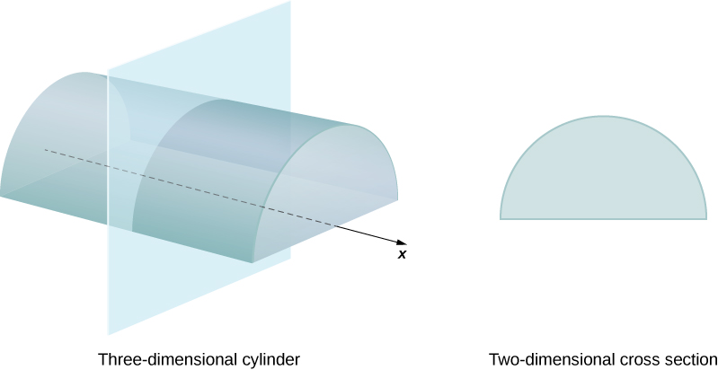
$This graphic has two figures. The first figure is half of a cylinder, on the flat portion. The cylinder has a line through the center labeled “x”. Vertically cutting through the cylinder, perpendicular to the line is a plane. The second figure is a two dimensional cross section of the cylinder intersecting with the plane. It is a semi-circle.$
Figure $\PageIndex{1}$: Each cross-section of a particular cylinder is identical to the others.

If a solid does not have a constant cross-section (and it is not one of the other basic solids), we may not have a formula for its volume. In this case, we can use a definite integral to calculate the volume of the solid. We do this by slicing the solid into pieces, estimating the volume of each slice, and then adding those estimated volumes together. The slices should all be parallel to one another, and when we put all the slices together, we should get the whole solid. Consider, for example, the solid $S$ shown in Figure $\PageIndex{2}$, extending along the $x$-axis.

$This figure is a graph of a 3-dimensional solid. It has one edge along the x-axis. The x-axis is part of the 2-dimensional coordinate system with the y-axis labeled. The edge of the solid along the x-axis starts at a point labeled “a” and stops at a point labeled “b”.$
Figure $\PageIndex{2}$: A solid with a varying cross-section.

We want to divide $S$ into slices perpendicular to the $x$-axis. As we see later in the chapter, there may be times when we want to slice the solid in some other direction - say, with slices perpendicular to the $y$-axis. The decision of which way to slice the solid is vital. If we make the wrong choice, the computations can get quite messy. Later in the chapter, we examine some of these situations in detail and decide which way to slice the solid. For the purposes of this section, however, we use slices perpendicular to the $x$-axis.

Because the cross-sectional area is not constant, we let $A(x)$ represent the cross-sectional area of the cross-section at point $x$. Now let $P=\{x_0,x_1,\ldots,x_n\}$ be a regular partition of $[a,b]$, and for $i=1,2,\ldots,n$, let $S_i$ represent the slice of $S$ stretching from $x_{i−1}$ to $x_i$. The following figure shows the sliced solid with $n=3$.

$This figure is a graph of a 3-dimensional solid. It has one edge along the x-axis. The x-axis is part of the 2-dimensional coordinate system with the y-axis labeled. The edge of the solid along the x-axis starts at a point labeled “a=xsub0”. The solid is divided up into smaller solids with slices at xsub1, xsub2, and stops at a point labeled “b=xsub3”. These smaller solids are labeled Ssub1, Ssub2, and Ssub3. They are also shaded.$
Figure $\PageIndex{3}$: The solid $S$ has been divided into three slices perpendicular to the $x$-axis.

Finally, for $i=1,2,\ldots,n$, let $x^∗_i$ be an arbitrary point in $[x_{i−1},x_i]$. Then the volume of slice $S_i$ can be estimated by $V(S_i) \approx A(x^∗_i)\, \Delta x$. Adding these approximations together, we see the volume of the entire solid $S$ can be approximated by\[V(S) \approx \sum_{i=1}^nA(x^∗_i)\, \Delta x. \nonumber \]By now, we can recognize this as a Riemann sum, and our next step is to take the limit as $n \to \infty .$ Then we have\[V(S)=\lim_{n \to \infty }\sum_{i=1}^nA(x^∗_i)\, \Delta x= \int _a^b A(x)\,dx. \nonumber \]The technique we have just described is called the slicing method. To apply it, we use the following strategy.

Problem-Solving Strategy: Finding Volumes by the Slicing Method

Examine the solid and determine the shape of a cross-section of the solid. It is often helpful to draw a picture if one is not provided.
Determine a formula for the area of the cross-section.
Integrate the area formula over the appropriate interval to get the volume.

This section assumes the slices are perpendicular to the $x$-axis. Therefore, the area formula is in terms of $x$, and the limits of integration lie on the $x$-axis. However, the problem-solving strategy shown here is valid regardless of how we choose to slice the solid.

Example $\PageIndex{1}$

We know from Geometry that the formula for the volume of a pyramid is $V=\frac{1}{3}Ah$. If the pyramid has a square base, this becomes $V=\frac{1}{3}a^2h$, where $a$ denotes the length of one side of the base. We are going to use the slicing method to derive this formula.

Solution

We want to apply the slicing method to a pyramid with a square base. To set up the integral, consider the pyramid shown in Figure $\PageIndex{4}$, oriented along the $x$-axis.

$This figure has two graphs. The first graph, labeled “a”, is a pyramid on its side. The x-axis goes through the middle of the pyramid. The point of the top of the pyramid is at the origin of the x y coordinate system. The base of the pyramid is shaded and labeled “a”. Inside of the pyramid is a shaded rectangle labeled “s”. The distance from the y-axis to the base of the pyramid is labeled “h”. the distance the rectangle inside of the pyramid to the y-axis is labeled “x”. The second figure is a cross section of the pyramid with the x and y axes labeled. The cross section is a triangle with one side labeled “a”, perpendicular to the x-axis. The distance a is from the y-axis is h. There is another perpendicular line to the x-axis inside of the triangle. It is labeled “s”. It is x units from the y-axis.$
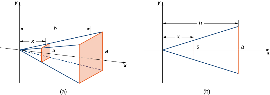
Figure $\PageIndex{4}$: (a) A pyramid with a square base is oriented along the $x$-axis. (b) A two-dimensional view of the pyramid is seen from the side.

We first want to determine the shape of a cross-section of the pyramid. We know the base is a square, so the cross-sections are squares as well. Now, we want to determine a formula for the area of one of these cross-sectional squares. Looking at Figure $\PageIndex{4}$(b), and using a proportion, since these are similar triangles, we have\[\dfrac{s}{a}=\dfrac{x}{h} \nonumber \]or\[s=\dfrac{ax}{h}. \nonumber \]Therefore, the area of one of the cross-sectional squares is\[A(x)=s^2=\left(\dfrac{ax}{h}\right)^2. \nonumber \]Then we find the volume of the pyramid by integrating from $0$ to $h$:\[V= \int _0^hA(x)\,dx= \int _0^h\left(\dfrac{ax}{h}\right)^2\,dx=\dfrac{a^2}{h^2} \int _0^hx^2\,dx=\Big[\dfrac{a^2}{h^2}\left(\dfrac{1}{3}x^3\right)\Big]\bigg|^h_0=\dfrac{1}{3}a^2h. \nonumber \]This is the formula we were looking for.

Checkpoint $\PageIndex{1}$

Use the slicing method to derive the formula \[V=\frac{1}{3} \pi r^2h \nonumber \] for the volume of a circular cone.

Hint: Use similar triangles, as in Example $\PageIndex{1}$.

While Example $ \PageIndex{1} $ is a shape we are familiar with, it behooves us to experiment with finding the volume of a solid having a more challenging design. For this discussion, we consider solids having a base region defined by a given boundary. This boundary is often an area between two functions on a specified interval, however, it can be a region bounded by a non-functional curve such as a conic section. Onto this base region, we will slide in cross-sectional slices perpendicular to the base (see the Interactive Element below).

Interactive Element: Volumes of Known Cross-sections

Description: This Geogebra applet allows you to visualize how a solid of known cross-sections is generated by placing cross-sectional slices perpendicular to the $ x $-axis on a base defined by the boundary between two functions (red and blue) from $ x = 0 $ to $ X $, where you can adjust $ X $ using the bottom slider.

Interact: Adjust the rightmost boundary, $ X $, of the region to whatever value you want, select a single cross-sectional shape (square, equilateral triangle, or semi-circle), increase $ n $ to a decent number of slices to help you visualize what is going on, and (finally) use your mouse to adjust the graph of the right side of the applet to see the resulting solid.

Let's take a look at two examples.

Example $\PageIndex{2}$

Find the volume of the solid with base region bounded by $ f(x) = 4 - x^2 $ and the $ x $-axis, where the cross-sections perpendicular to the $ x $-axis are isosceles right triangles with hypotenuse in the base region.

Solution

We begin by drawing a top-down view of the base region, including the $ i^{\text{th}} $ slice (see Figure $ \PageIndex{5} $ below).

$Math401_1_2_2A.png$
Figure $ \PageIndex{5} $: A top-down view of the base region along with the $ i^{\text{th}} $ slice.

It will also be beneficial to sketch a side view of the $ i^{\text{th}} $ slice (see Figure $ \PageIndex{6} $ below).

$Math401_1_2_2B_Fix01.png$
Figure $ \PageIndex{6} $: A side view of the $ i^{\text{th}} $ slice.

The volume of this $ i^{\text{th}} $ slice can be found using the fact that the surface area of a triangle is one-half the product of the base and the height. Hence,\[ V_i = \dfrac{1}{2} \left(\text{base}\right)\left(\text{height}\right) \Delta x = \dfrac{1}{2} \left( f(x_i^*) - 0 \right) \left(\text{height}\right) \Delta x = \dfrac{1}{2} \left( 4 - (x_i^*)^2 \right) \left(\text{height}\right) \Delta x. \nonumber \]To determine the height of this $ i^{\text{th}} $ slice, we use the fact that the base has length $ 4 - (x_i^*)^2 $, which means half of the base has length $ \frac{1}{2}\left(4 - (x_i^*)^2\right) $. Since the triangle is an isosceles right triangle, the height equals this half-base length. Hence,\[ V_i = \dfrac{1}{4} \left( 4 - (x_i^*)^2 \right)^2 \Delta x. \nonumber \]From Figure $ \PageIndex{5} $, we can see that symmetry can be used so that we only need to add up the volumes of the slices starting at $ x = 0 $ and ending at $ x = 2 $. We double this result to approximate the total area. That is,\[ V \approx 2 \sum_{i = 0}^n V_i = \dfrac{1}{2} \sum_{i = 0}^n \left( 4 - (x_i^*)^2 \right)^2 \Delta x. \nonumber \]Taking the limit as $ n \to \infty $, we get\[ \begin{array}{rcl}
V & = & \dfrac{1}{2} \displaystyle \int_0^2 (4 - x^2)^2 \, dx \\
\\
& = & \dfrac{1}{2} \displaystyle \int_0^2 16 - 8 x^2 + x^4 \, dx \\
\\
& = & \dfrac{1}{2} \left( 16x - \dfrac{8}{3} x^3 + \dfrac{1}{5} x^5 \right) \bigg|_0^2 \\
\\
& = & \dfrac{1}{2} \left( 32 - \dfrac{64}{3} + \dfrac{32}{5} \right) \\
\\
& = & \dfrac{128}{15} \, \text{cubic units} \\
\end{array} \nonumber \]

Example $\PageIndex{3}$

Find the volume of the solid with base region bounded by $ f(x) = 4 - x^2 $ and the $ x $-axis, where the cross-sections perpendicular to the $ y $-axis are semi-circles.

Solution

Just as we did in Example $ \PageIndex{2} $, we begin by sketching a top-down view of the base region with the $ i^{\text{th}} $ slice, and a side view of the $ i^{\text{th}} $ slice (see Figure $ \PageIndex{7} $).

$Math401_1_2_3A.png$ $Math401_1_2_3B.png$
Figure $ \PageIndex{7} $A: A top-down view of the base region along with the $ i^{\text{th}} $ slice, and
Figure $ \PageIndex{7} $B: A side view of the $ i^{\text{th}} $ slice.

The volume of the $ i^{\text{th}} $ slice is\[ V_i = \dfrac{1}{2} \pi \left(r_i^*\right)^2 \Delta y = \dfrac{1}{2} \pi \left( x_i^* \right)^2 \Delta y. \nonumber \]Using the relation $ y_i^* = 4 - \left(x_i^*\right)^2 $, we get\[ V_i = \dfrac{1}{2} \pi \left( 4 - y_i^* \right) \Delta y. \nonumber \]Therefore\[ \begin{array}{rcl}
V & = & \displaystyle \lim_{n \to \infty} \sum_{i = 0}^n V_i \\
\\
& = & \displaystyle \int_{y = 0}^{y = 4} \dfrac{1}{2} \pi \left( 4 - y \right) \, dy \\
\\
& = & \dfrac{\pi}{2} \left( 4y - \dfrac{y^2}{2} \right) \bigg|_{y = 0}^{y = 4} \\
\\
& = & 4 \pi \, \text{cubic units} \\
\end{array} \nonumber \]

Search

Text Color

Text Size

Margin Size

Font Type

Problem-Solving Strategy: Finding Volumes by the Slicing Method

Example \(\PageIndex{1}\)

Checkpoint \(\PageIndex{1}\)

Interactive Element: Volumes of Known Cross-sections

Example \(\PageIndex{2}\)

Example \(\PageIndex{3}\)