2.5: Numerical Integration

Note to the Instructor (click to expand) We finally get to the final frontier of integration techniques. All of this is core content for Calculus II. To succeed in this section, you'll need to use some skills from previous courses. While you should already know them, this is the first time they've been required. You can review these skills in CRC's Corequisite Codex. If you have a support class, it might cover some, but not all, of these topics. Prerequisite Skills and Support Topics (click to expand) Graphing Functions Local and Absolute Extrema: Finding the error bounds for the Midpoint, Trapezoidal, and Simpson's Rules requires finding the absolute maximum value of a function's second or fourth derivative over a closed interval  The following is a list of learning objectives for this section. Learning Objectives (click to expand) Approximate the value of a definite integral by using the Midpoint and Trapezoidal Rules. Determine the absolute and relative error in using a numerical integration technique. Estimate the absolute and relative error using an error-bound formula. Recognize when the midpoint and Trapezoidal Rules over- or underestimate the true value of an integral. Use Simpson's Rule to approximate the value of a definite integral to a given accuracy.

Hawk A.I. Section-Specific Tutor To access the Hawk A.I. Tutor, you will need to be logged into your campus Gmail account.

The antiderivatives of many functions either cannot be expressed or cannot be expressed easily in closed form (that is, in terms of known functions). Consequently, rather than directly evaluating definite integrals of these functions, we resort to various numerical integration techniques to approximate their values. In this section, we explore several of these techniques. In addition, we examine the process of estimating the error when using these techniques.

The Midpoint Rule

Earlier in this text, we defined the definite integral of a function over an interval as the limit of Riemann sums. In general, any Riemann sum of a function \( f(x)\) over an interval \([a,b]\) may be viewed as an estimate of \(\displaystyle \int ^b_af(x)\, dx\). Recall that a Riemann sum of a function \( f(x)\) over an interval \( [a,b]\) is obtained by selecting a partition\[ P=\{x_0,x_1,x_2, \ldots ,x_n\}, \nonumber \]where \(a = x_0 \lt x_1 \lt x_2 \lt \cdots \lt x_n = b \), and a set\[ S=\{x^*_1,x^*_2, \ldots ,x^*_n\}, \nonumber \]where \(x_{i−1} \leq x^*_i \leq x_i \text{ for all } \, i = 1, 2, \ldots, n.\)

The Riemann sum corresponding to the partition \(P\) and the set \(S\) is given by\[ \sum^n_{i=1}f(x^*_i) \Delta x_i, \nonumber \]where \( \Delta x_i = x_i − x_{i−1}\) is the length of the \( i^{\text{th}}\) subinterval.

In Differential Calculus, we learned the Left Endpoint and Right Endpoint approximation methods for estimating the value of a definite integral. The Midpoint Rule for estimating the value of a definite integral uses a Riemann sum with subintervals of equal width and the midpoints, \( m_i\), of each subinterval in place of \( x^*_i\). Formally, we state a theorem regarding the convergence of the Midpoint Rule as follows.

Theorem: Midpoint Rule

Let \( f(x)\) be continuous on \([a,b]\), \( n\) be a positive integer, and \( \Delta x=\frac{b−a}{n}\). If \( [a,b]\) is divided into \( n\) subintervals, each of length \( \Delta x\), and \( m_i = \frac{x_{i - 1} + x_i}{2}\) is the midpoint of the \( i^{\text{th}}\) subinterval, set\[M_n = \sum_{i=1}^n f(m_i) \Delta x = \sum_{i=1}^n f\left(\dfrac{x_{i - 1} + x_i}{2}\right) \Delta x. \nonumber \]Then\[ \lim_{n \to \infty } M_n = \int ^b_af(x)\,dx.\nonumber \]

As we can see in Figure \(\PageIndex{1}\), if \( f(x) \geq 0\) over \( [a,b]\), then \(\displaystyle \sum^n_{i=1}f(m_i) \Delta x\) corresponds to the sum of the areas of rectangles approximating the area between the graph of \( f(x)\) and the \(x\)-axis over \([a,b]\). The graph shows the rectangles corresponding to \(M_4\) for a nonnegative function over a closed interval \([a,b]\).

Figure \(\PageIndex{1}\): The Midpoint Rule approximates the area between the graph of \(f(x)\) and the \(x\)-axis by summing the areas of rectangles with midpoints that are points on \(f(x)\).

If we are lucky enough to know the exact value of a definite integral, then we can define the absolute error of an estimation as follows:

Definition: Absolute Error

The absolute error, \( E_* \), of a numerical approximation, \( A \), to the true value of the quantity, \( T \), is defined to be\[ E_* = |T - A|. \nonumber \]The notation "\( * \)" is reserved for the method being used. For example, the absolute error if using the Midpoint Rule with \( n = 10 \) to approximate the value of a definite integral is\[ E_M = \left| T - M_{10} \right|. \nonumber \]

Example \(\PageIndex{1}\): Using the Midpoint Rule with \(M_4\)

Use the Midpoint Rule to estimate\[ \int ^1_0x^2\,dx \nonumber \]using four subintervals. Compare the result with the actual value of this integral.

Solution

Each subinterval has length \( \Delta x=\frac{1−0}{4}=\frac{1}{4}\). Therefore, the subintervals consist of\[\left[0,\dfrac{1}{4}\right], \, \left[\dfrac{1}{4},\dfrac{1}{2}\right], \, \left[\dfrac{1}{2},\dfrac{3}{4}\right], \, \text{and} \, \left[\dfrac{3}{4},1\right].\nonumber \]The midpoints of these subintervals are \(\left\{\frac{1}{8},\,\frac{3}{8},\,\frac{5}{8},\, \frac{7}{8}\right\}\). Thus,\[\begin{array}{rcl}
M_4 & = & \dfrac{1}{4}\cdot f\left(\dfrac{1}{8}\right)+\dfrac{1}{4}\cdot f\left(\dfrac{3}{8}\right)+\dfrac{1}{4}\cdot f\left(\dfrac{5}{8}\right)+\dfrac{1}{4}\cdot f\left(\dfrac{7}{8}\right) \\[16pt]
& = & \dfrac{1}{4} \cdot \dfrac{1}{64}+\dfrac{1}{4} \cdot \dfrac{9}{64}+\dfrac{1}{4} \cdot \dfrac{25}{64}+\dfrac{1}{4} \cdot \dfrac{49}{64}\\[16pt]
& = & \dfrac{21}{64} \\[16pt]
& = & 0.328125. \\[16pt]
\end{array} \nonumber \]Since the true value of this definite integral is\[ T = \int ^1_0x^2\, dx = \dfrac{1}{3},\nonumber \]the absolute error in this approximation is\[ E_M = \left| T - M_4\right| = \left| \dfrac{1}{3} − \dfrac{21}{64}\right| = \dfrac{1}{192} \approx 0.0052, \nonumber \]and we see that the Midpoint Rule produces an estimate that is somewhat close to the actual value of the definite integral.

Example \(\PageIndex{2}\): Using the Midpoint Rule with \(M_6\)

Use \(M_6\) to estimate the length of the curve\[y=\dfrac{1}{2}x^2, \nonumber \]on \([1,4]\).

Solution

The length of \(y=\frac{1}{2}x^2\) on \([1,4]\) is\[s = \int ^4_1 \sqrt{1+\left(\dfrac{dy}{dx}\right)^2}\,dx.\nonumber \]Since \(\frac{dy}{dx} = x\), this integral becomes \(\displaystyle \int ^4_1\sqrt{1+x^2}\,dx.\)

If \([1,4]\) is divided into six subintervals, then each subinterval has length \( \Delta x=\frac{4−1}{6}=\frac{1}{2}\). The midpoints of the subintervals are \(\left\{\frac{5}{4},\frac{7}{4},\frac{9}{4},\frac{11}{4},\frac{13}{4},\frac{15}{4}\right\}\). If we set \(f(x)=\sqrt{1+x^2}\), we get\[\begin{array}{rcl}
M_6 & = & \dfrac{1}{2}\cdot f\left(\dfrac{5}{4}\right)+\dfrac{1}{2}\cdot f\left(\dfrac{7}{4}\right)+\dfrac{1}{2}\cdot f\left(\dfrac{9}{4}\right)+\dfrac{1}{2}\cdot f\left(\dfrac{11}{4}\right)+\dfrac{1}{2}\cdot f\left(\dfrac{13}{4}\right)+\dfrac{1}{2}\cdot f\left(\dfrac{15}{4}\right) \\[16pt]
& \approx & \dfrac{1}{2}(1.6008+2.0156+2.4622+2.9262+3.4004+3.8810) \\[16pt]
& = & 8.1431 \, \text{ units}. \\[16pt]
\end{array} \nonumber \]

Checkpoint \(\PageIndex{2}\)

Use \( M_2 \) to estimate\[ \int ^2_1\dfrac{1}{x}\,dx. \nonumber \]

Answer

\(\frac{24}{35}\approx 0.685714\)

The Trapezoidal Rule

We can also approximate the value of a definite integral by using trapezoids rather than rectangles (see Figure \(\PageIndex{2}\)).

Figure \(\PageIndex{2}\): Trapezoids may be used to approximate the area under a curve, hence approximating the definite integral.

The Trapezoidal Rule for estimating definite integrals uses trapezoids rather than rectangles to approximate the area under a curve. Consider the trapezoids in Figure \(\PageIndex{2}\) to gain insight into the rule's final form. We assume that the length of each subinterval is given by \( \Delta x\). First, recall that the area of a trapezoid with a height of \(h\) and bases of length \(b_1\) and \(b_2\) is given by\[\text{Area}=\dfrac{1}{2}h(b_1+b_2). \nonumber \]We see that the first trapezoid has a "height" \( \Delta x\) and parallel "bases" of length \( f(x_0)\) and \( f(x_1)\). Thus, the area of the first trapezoid in Figure \(\PageIndex{2}\) is\[ \dfrac{1}{2} \Delta x \left(f(x_0)+f(x_1)\right).\nonumber \]The areas of the remaining three trapezoids are\[ \dfrac{1}{2} \Delta x \left((f(x_1)+f(x_2)\right),\, \dfrac{1}{2} \Delta x \left(f(x_2)+f(x_3)\right), \text{ and } \dfrac{1}{2} \Delta x \left(f(x_3)+f(x_4)\right). \nonumber \]Consequently,\[ \int ^b_af(x)\,dx \approx \dfrac{1}{2} \Delta x \left(f(x_0)+f(x_1)\right)+\dfrac{1}{2} \Delta x \left(f(x_1)+f(x_2)\right) + \dfrac{1}{2} \Delta x \left(f(x_2) + f(x_3)\right) + \dfrac{1}{2} \Delta x\left(f(x_3)+f(x_4)\right).\nonumber \]After taking out a common factor of \(\frac{1}{2} \Delta x\) and combining like terms, we have\[ \int ^b_af(x)\,dx \approx \dfrac{\Delta x}{2}\left[f(x_0)+2 f(x_1)+2 f(x_2)+2 f(x_3)+f(x_4)\right].\nonumber \]Generalizing, we formally state the following rule.

Theorem: The Trapezoidal Rule

Let \(f(x)\) be continuous over \([a,b]\), \(n\) be a positive integer, and \( \Delta x=\frac{b−a}{n}\). If \( [a,b]\) is divided into \(n\) subintervals, each of length \( \Delta x\), with endpoints at \( P=\{x_0,x_1,x_2, \ldots ,x_n\}\), set\[T_n=\dfrac{ \Delta x}{2}\left[f(x_0)+2 f(x_1) + 2 f(x_2) + \cdots + 2 f(x_{n−1}) + f(x_n)\right]. \nonumber \]Then,\[ \lim_{n \to \infty}T_n = \int ^b_af(x)\,dx. \nonumber \]

Before continuing, let's make a few observations about the Trapezoidal Rule. First of all, it is useful to note that\[T_n=\dfrac{1}{2}(L_n+R_n), \text{ where } L_n = \sum_{i=1}^nf(x_{i−1}) \Delta x \text{ and } R_n=\sum_{i=1}^nf(x_i) \Delta x. \nonumber \]That is, the Trapezoidal Rule is the average of the Left Endpoint Approximation, \(L_n\), and the Right Endpoint Approximation, \(R_n\). In addition, a careful examination of Figure \(\PageIndex{3}\) (see below) leads us to make the following observations about using the Trapezoidal Rules and Midpoint Rules to estimate the definite integral of a nonnegative function. The Trapezoidal Rule tends to overestimate the value of a definite integral systematically over intervals where the function is concave up and to underestimate the value systematically over intervals where the function is concave down. On the other hand, the Midpoint Rule averages out these errors somewhat by partially overestimating and underestimating the value of the definite integral over these same types of intervals. This leads us to hypothesize that, in general, the Midpoint Rule tends to be more accurate than the Trapezoidal Rule.

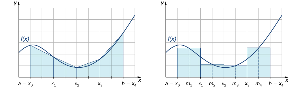
Figure \(\PageIndex{3}\): The Trapezoidal Rule tends to be less accurate than the Midpoint Rule.

Example \(\PageIndex{3}\): Using the Trapezoidal Rule

Use the Trapezoidal Rule to estimate\[ \int ^1_0x^2\,dx \nonumber \]using four subintervals.

Solution

The endpoints of the subintervals consist of elements of the set \(P=\left\{0,\frac{1}{4},\, \frac{1}{2},\, \frac{3}{4},1\right\}\) and \( \Delta x=\frac{1−0}{4}=\frac{1}{4}.\) Thus,\[\begin{array}{rcl}
\displaystyle \int^1_0 x^2 \, dx & \approx & \dfrac{1}{2} \cdot \dfrac{1}{4} \left[f(0)+2 f\left(\dfrac{1}{4}\right)+2 f\left(\dfrac{1}{2}\right)+2 f\left(\dfrac{3}{4}\right)+f(1)\right] \\[16pt]
& = & \dfrac{1}{8}\left(0+2 \cdot \dfrac{1}{16}+2 \cdot \dfrac{1}{4}+2 \cdot \dfrac{9}{16}+1\right) \\[16pt]
& = & \dfrac{11}{32} \\[16pt]
& = & 0.34375 \\[16pt]
\end{array} \nonumber \]

Checkpoint \(\PageIndex{3}\)

Use \( T_2 \) to estimate\[ \int ^2_1\dfrac{1}{x}\,dx. \nonumber \]

Answer

\(\frac{17}{24} \approx 0.708333\)

Absolute and Relative Error

An important aspect to consider when using numerical integration techniques is calculating their errors from the true value of their associated definite integrals. As mentioned, a method's absolute error is given by\[ E_* = \left| T - A \right|. \nonumber \]Another important measure is the relative error of an approximation.

Definition: Relative Error

The relative error of an approximation is the error as a percentage of the actual value and is given by\[\left| \dfrac{T − A_*}{T}\right| \cdot 100\% = \dfrac{E_*}{|T|} \cdot 100\%. \nonumber \]

Example \(\PageIndex{4}\): Calculating Error in the Midpoint Rule

Calculate the relative error in the estimate of \(\displaystyle \int ^1_0x^2\,dx\) using the Midpoint Rule, found in Example \(\PageIndex{1}\).

Solution

We computed the absolute error to be \( E_M = \frac{1}{192} \approx 0.0052\). Therefore, the relative error is\[ \left| \dfrac{T - M_4}{T} \right| = \dfrac{E_M}{|T|} = \dfrac{1/192}{1/3}=\dfrac{1}{64} \approx 0.015625 \approx 1.6\%.\nonumber \]

Example \(\PageIndex{5}\): Calculating Error in the Trapezoidal Rule

Calculate the absolute and relative error in the estimate of \(\displaystyle \int ^1_0x^2\,dx\) using the Trapezoidal Rule, found in Example \(\PageIndex{3}\).

Solution

The true value is \(\displaystyle \int ^1_0x^2\,dx=\frac{1}{3}\), and our estimate from the example is \(T_4=\frac{11}{32}\). Thus, the absolute error is given by\[ E_T = \left| T - T_4 \right| = \left|\dfrac{1}{3}−\dfrac{11}{32}\right| = \dfrac{1}{96} \approx 0.0104. \nonumber \]The relative error is given by\[\left| \dfrac{T − T_4}{T}\right| = \dfrac{E_T}{|T|} = \dfrac{1/96}{1/3} = 0.03125 \approx 3.1\%.\nonumber \]

Checkpoint \(\PageIndex{5}\)

In an earlier checkpoint, we estimated \(\displaystyle \int ^2_1\frac{1}{x}\,dx\) to be \(\frac{24}{35}\) using \(M_2\). The actual value of this integral is \(\ln 2\). Using \(\frac{24}{35} \approx 0.6857\) and \(\ln 2 \approx 0.6931\), calculate the absolute error and the relative error.

Answer

The absolute error is \(\approx 0.0074\), and the relative error is \(\approx 1.1\%\).

Error Bounds on the Midpoint and Trapezoidal Rules

In the two previous examples, we could compare our estimate of an integral with the actual value of the integral; however, we do not typically have this luxury. In general, if we are approximating an integral, we are doing so because we cannot easily compute the exact value of the integral. Therefore, determining an upper bound for the error in an approximation of an integral is often helpful. The following theorem provides error bounds for the Midpoint and Trapezoidal Rules. The theorem is stated without proof.¹

Theorem: Error Bounds for the Midpoint and Trapezoidal Rules

Let \(f(x)\) be a continuous function over \([a,b]\), where \(f^{\prime\prime}(x)\) exists over this same interval interval. If \(M\) is the maximum value of \(\left|f^{\prime\prime}(x)\right|\) over \([a,b]\), then the upper bounds for the error in using \(M_n\) and \(T_n\) to estimate \(\displaystyle \int ^b_af(x)\, dx\) are

\[E_M \leq \dfrac{M(b−a)^3}{24n^2} \label{MidError} \]

and

\[E_T \leq \dfrac{M(b−a)^3}{12n^2}. \label{TrapError} \]

We can use these bounds to determine the value of \(n\) necessary to guarantee that the error in an estimate is less than a specified value.

Example \(\PageIndex{6}\): Determining the Number of Intervals to Use

What value of \(n\) should be used to guarantee that an estimate of

\[ \int ^1_0e^{x^2}\,dx \nonumber \]

is accurate to within \(0.01\) if we use the Midpoint Rule?

Solution

We begin by determining the value of \(M\), the maximum value of \( \left|f^{\prime\prime}(x)\right|\) over \( [0,1]\) for \( f(x)=e^{x^2}\).

Since \( f^{\prime}(x)=2xe^{x^2},\) we have

\[ f^{\prime\prime}(x)=2e^{x^2}+4x^2e^{x^2}.\nonumber \]

Thus,

\[ \left|f^{\prime\prime}(x)\right| = 2e^{x^2}(1+2x^2) \leq 2 \cdot e \cdot 3 = 6e.\nonumber \]

From the error-bound Equation \(\ref{MidError}\), we have

\[ E_M \leq \dfrac{M(b−a)^3}{24n^2} \leq \dfrac{6e(1−0)^3}{24n^2}=\dfrac{6e}{24n^2}.\nonumber \]

Now we solve the following inequality for \(n\):

\[\dfrac{6e}{24n^2} \leq 0.01.\nonumber \]

Thus, \(n \geq \sqrt{\frac{600e}{24}} \approx 8.24\). Since \(n\) must be an integer satisfying this inequality, a choice of \(n=9\) would guarantee that

\[ E_M = \left|T - M_n \right| = \left| \int ^1_0e^{x^2}\,dx − M_n \right| \lt 0.01.\nonumber \]

Analysis

We might have been tempted to round \(8.24\) down and choose \(n=8\), but this would be incorrect because we must have an integer greater than or equal to \(8.24\). We must remember that the error estimates provide an upper bound only for the error. The actual estimate may be a much better approximation than the error bound indicates.

Checkpoint \(\PageIndex{6}\)

Use Equation \(\ref{MidError}\) to find an upper bound for the error in using \(M_4\) to estimate \(\displaystyle \int ^1_0x^2\,dx.\)

Answer

\(\frac{1}{192}\)

Simpson's Rule

With the Midpoint Rule, we estimated areas of regions under curves by using rectangles. In a sense, we approximated the curve with piecewise constant functions. With the Trapezoidal Rule, we approximated the curve using piecewise linear functions. What if we were to approximate a curve using piecewise quadratic functions instead? With Simpson's Rule, we do just this. Consider the function in Figure \( \PageIndex{ 4 } \).

Figure \( \PageIndex{ 4 } \)

We partition the interval into an even number of subintervals of equal width (the necessity of the even number of subintervals will be revealed shortly). If we wish to string together quadratic functions to help us approximate the area under this curve, we face a new challenge - the Left Endpoint, Right Endpoint, Midpoint, and Trapezoidal Rules each required "tops" to our slices that were linear functions (horizontal lines in all cases but the Trapezoidal Rule). Since we only need two points to build a line, we only needed our subintervals to include neighboring points in the partition - namely, \( \left(x_{i - 1},f(x_{i - 1})\right) \) and \( \left(x_i, f(x_i)\right) \). This is why the \( i^{\text{th}} \) subinterval was \( \left[ x_{i - 1}, x_i \right] \) in each of these methods; however, quadratic functions graph as parabolas, and from our Algebra, we know we need three points to find the equation of a parabola. Hence, we need an "expanded" interval containing three neighboring points to uniquely find the approximating parabola, as see in Figure \( \PageIndex{ 5 } \).

Figure \( \PageIndex{ 5 } \)

Our goal is to derive a formula for the area of this \( i^{\text{th}} \) slice over the interval \( [x_{i - 1}, x_{i + 1}] \). Before continuing, let's make sure we all agree that the red points in Figure \( \PageIndex{ 5 } \) are \( \left( x_{i-1}, f(x_{i - 1}) \right) \), \( \left( x_{i}, f(x_{i}) \right) \), and \( \left( x_{i+1}, f(x_{i + 1}) \right) \). For notational simplicity, let's replace those function values with a cleaner notation - \( \left( x_{i - 1}, y_{i - 1} \right) \), \( \left( x_{i}, y_{i} \right) \), and \( \left( x_{i + 1}, y_{i + 1} \right) \).

There are several ways to approach this, however, we will use the simple concept that shifting a function left or right does not affect the area between the function and the \( x \)-axis (another way to say this is that the area under the curve on a given interval is invariant under horizontal translations). Therefore, we shift the function so \( x_i = 0 \) and temporarily let \( h = \Delta x  \). Figure \( \PageIndex{ 6 } \) reflects this change.

Figure \( \PageIndex{ 6 } \)

As mentioned, computationally, this shift has no effect; however, it simplifies our derivation quite a bit. The most important part we note is that the \( y \)-values of those points are still \( y_{i - 1} \), \( y_i \), and \( y_{i + 1} \). Thus, the three red points in Figure \( \PageIndex{ 6 } \) are \( \left( -h, y_{i - 1} \right) \), \( \left( 0, y_{i} \right) \), and \( \left( h, y_{i + 1} \right) \). We know the equation of a parabola is\[ y = Ax^2 + Bx + C. \nonumber \]Substituting in the three points, we get the equations\[ \begin{array}{rcl}
y_{i - 1} & = & Ah^2 - Bh + C \\
y_i & = & C \\
y_{i + 1} & = & Ah^2 + Bh + C \\
\end{array}
\label{tempeqns} \]We now turn our focus to computing the approximated area under \( f \) on the interval \( \left[ x_{i - 1}, x_{i+1} \right] \).\[ \text{Area of the }i^{\text{th}} \text{ slice} \approx \int_{x_{i - 1}}^{x_{i  + 1}} Ax^2 + Bx + C \, dx = \int_{-h}^{h} Ax^2 + Bx + C \, dx = \left( \left. \dfrac{A}{3} x^3 + \dfrac{B}{2} x^2 + Cx \right) \right|_{-h}^{h} = \dfrac{2A}{3} h^3 + 2Ch = \dfrac{h}{3} \left( 2 A h^2 + 6 C \right). \nonumber \]A little ingenuity reveals that the expression \( 2 A h^2 + 6 C \) is a combination of the equations in \ref{tempeqns}. Specifically, if you took one of the first equation, four of the second, and one of the third, you would get\[ \begin{array}{lrcl}
& y_{i - 1} & = & Ah^2 - Bh + C \\
& 4y_i & = & 4C \\
+ & y_{i + 1} & = & Ah^2 + Bh + C \\
\hline & y_{i-1} + 4y_i + y_{i + 1} & = & 2Ah^2 + 6C \\
\end{array} \nonumber \]Does this look familiar? I hope so because we just spent a little while deriving that right side! This leads to a clean approximation to the area of the \( i^{\text{th}} \) slice:\[ \text{Area of the }i^{\text{th}} \text{ slice} \approx \dfrac{h}{3} \left( 2 A h^2 + 6 C \right) = \dfrac{h}{3}\left( y_{i-1} + 4y_i + y_{i + 1} \right) = \dfrac{h}{3}\left( f(x_{i-1}) + 4 f(x_i) + f(x_{i + 1}) \right). \nonumber \]Now that we have an explicit formula for the area of the \( i^{\text{th}} \) slice, we can use a Riemann sum to approximate the area under the curve from \( x_0 \) to \( x_n \). Before we setup the summation, however, it is important to visualize that the edges of the \( i^{\text{th}} \) slice occur at \( x = x_{i - 1} \) and \( x_{i + 1} \). Hence, our summation will go from \( i = 1 \) to \( i = n - 1 \) (the \( (n - 1)^{\text{st}} \) slice having \( x_n \) as its rightmost edge). Moreover, the center of the first slice is at \( x_1 \), the second at \( x_3 \), the third at \( x_5 \), and so on. The rightmost edge of the entire interval must be \( x_n \), where \( n \) is even (thus, the requirement for an even number of slices). Thus,\[ \begin{array}{rcl}
A & \approx & \left[ \dfrac{h}{3}\left( f(x_{0}) + 4 f(x_1) + f(x_{2}) \right) + \dfrac{h}{3}\left( f(x_{2}) + 4 f(x_3) + f(x_{4}) \right) + \dfrac{h}{3}\left( f(x_{4}) + 4 f(x_5) + f(x_{6}) \right) + \cdots \right. \\[16pt]
& & \quad \left. + \dfrac{h}{3}\left( f(x_{n-4}) + 4 f(x_{n - 3}) + f(x_{n - 2}) \right) + \dfrac{h}{3}\left( f(x_{n-2}) + 4 f(x_{n - 1}) + f(x_{n}) \right) \right] \\[16pt]
& = & \dfrac{h}{3}\left[ \left( f(x_{0}) + 4 f(x_1) + f(x_{2}) \right) + \left( f(x_{2}) + 4 f(x_3) + f(x_{4}) \right) + \left( f(x_{4}) + 4 f(x_5) + f(x_{6}) \right) + \cdots \right. \\[16pt]
& & \quad \left. + \left( f(x_{n-4}) + 4 f(x_{n - 3}) + f(x_{n - 2}) \right) + \left( f(x_{n-2}) + 4 f(x_{n - 1}) + f(x_{n}) \right) \right] \\[16pt]
& = & \dfrac{\Delta x}{3}\left[ \left( f(x_{0}) + 4 f(x_1) + f(x_{2}) \right) + \left( f(x_{2}) + 4 f(x_3) + f(x_{4}) \right) + \left( f(x_{4}) + 4 f(x_5) + f(x_{6}) \right) + \cdots \right. \\[16pt]
& & \left. + \left( f(x_{n-4}) + 4 f(x_{n - 3}) + f(x_{n - 2}) \right) + \left( f(x_{n-2}) + 4 f(x_{n - 1}) + f(x_{n}) \right) \right] \\[16pt]
& = & \dfrac{\Delta x}{3} \left( f(x_0) + 4 f(x_1) + 2f(x_2) + 4 f(x_3) + 2f(x_4) + \cdots +2 f(x_{n - 2}) + 4 f(x_{n - 1}) + f(x_n) \right) \\[16pt]
\end{array} \nonumber \]Other than the outer edges of the main interval, the doubling of the function values at even indexed partition values occurs because the edges of two parabolas meet there and their function values get double-counted. The general rule may be stated as follows.

Theorem: Simpson's Rule

Assume that \(f(x)\) is continuous over \([a,b]\). Let \(n\) be a positive even integer and \( \Delta x=\frac{b−a}{n}\). Let \([a,b]\) be divided into \(n\) subintervals, each of length \( \Delta x\), with endpoints at \(P=\{x_0,x_1,x_2, \ldots ,x_n\}\). Set\[S_n = \dfrac{\Delta x}{3}\left[f(x_0)+4f(x_1)+2f(x_2)+4f(x_3)+2f(x_4) + \cdots +2f(x_{n−2})+4f(x_{n−1})+f(x_n)\right]. \nonumber \]Then,\[\lim_{n \to \infty }S_n= \int ^b_af(x)\,dx.\nonumber \]

Just as the Trapezoidal Rule is the average of the Left Endpoint and Right Endpoint approximations for estimating definite integrals, Simpson's Rule may be obtained using a weighted average from the Midpoint and Trapezoidal Rules. It can be shown that \(S_{2n} = \left(\frac{2}{3}\right)M_n+\left(\frac{1}{3}\right)T_n\).

It is also possible to put a bound on the error when using Simpson's Rule to approximate a definite integral. The bound in the error is given by the following rule:

Theorem: Error Bound for Simpson's Rule

Let \(f(x)\) be a continuous function over \([a,b]\) having a fourth derivative, \( f^{(4)}(x)\), over this interval. If \(M\) is the maximum value of \(\left|f^{(4)}(x)\right|\) over \([a,b]\), then the upper bound for the error in using \(S_n\) to estimate \(\displaystyle \int ^b_af(x)\, dx\) is given by\[E_S \leq \dfrac{M(b−a)^5}{180n^4}. \nonumber \]

Example \(\PageIndex{7}\): Applying Simpson's Rule 1

Use \(S_2\) to approximate\[ \int ^1_0x^3\,dx. \nonumber \]Estimate a bound for the error in \(S_2\).

Solution

Since \([0,1]\) is divided into two intervals, each subinterval has length \( \Delta x=\frac{1−0}{2}=\frac{1}{2}\). The endpoints of these subintervals are \(\left\{0,\frac{1}{2},1\right\}\). If we set \(f(x)=x^3,\) then\[S_2 = \dfrac{1/2}{3} \left( f(0)+4 f\left(\dfrac{1}{2}\right)+f(1) \right) = \dfrac{1}{6} \left(0+4 \cdot \dfrac{1}{8}+1 \right) = \dfrac{1}{4}.\nonumber \]Since \( f^{(4)}(x)=0\) and consequently \(M=0,\) we see that\[ E_S \leq \dfrac{0(1)^5}{180 \cdot 2^4} = 0. \nonumber \]This bound indicates that the value obtained through Simpson's Rule is exact. A quick check will verify that, in fact, \(\displaystyle \int ^1_0x^3\,dx=\frac{1}{4}\).

Example \( \PageIndex{8}\): Applying Simpson's Rule 2

Use \(S_6\) to estimate the length of the curve\[y=\dfrac{1}{2}x^2 \nonumber \]over \([1,4]\)

Solution

The length of \(y=\frac{1}{2}x^2\) over \([1,4]\) is \(\displaystyle \int ^4_1\sqrt{1+x^2}\,dx\). If we divide \([1,4]\) into six subintervals, then each subinterval has length \( \Delta x=\frac{4−1}{6}=\frac{1}{2}\), and the endpoints of the subintervals are \( \left\{1,\frac{3}{2},2,\frac{5}{2},3,\frac{7}{2},4\right\}.\) Setting \( f(x)=\sqrt{1+x^2}\),\[ S_6 = \dfrac{1/2}{3} \left(f(1)+4f\left(\dfrac{3}{2}\right)+2f(2)+4f\left(\dfrac{5}{2}\right)+2f(3)+4f\left(\dfrac{7}{2}\right)+f(4)\right).\nonumber \]After substituting, we have\[S_6=\dfrac{1}{6} \left(1.4142+4 \cdot 1.80278+2 \cdot 2.23607+4 \cdot 2.69258+2 \cdot 3.16228+4 \cdot 3.64005+4.12311 \right) \approx 8.14594\,\text{units}. \nonumber \]

Checkpoint \(\PageIndex{8}\)

Use \(S_2\) to estimate\[ \int ^2_1\dfrac{1}{x}\,dx. \nonumber \]

Answer

\(\frac{25}{36} \approx 0.694444\)

---

Footnotes

¹ The exploration of numerical methods, their error bounds, and the trade-off between the accuracy of the method and its computational expense is the realm of a subfield of Mathematics called Numerical Analysis. If you are intrigued by how such methods (and their errors) are developed, I recommend taking a series of upper-division courses in Numerical Analysis.