
2.5: Numerical Integration
- Page ID
- 163273

\( \newcommand{\vecs}[1]{\overset { \scriptstyle \rightharpoonup} {\mathbf{#1}} } \)
\( \newcommand{\vecd}[1]{\overset{-\!-\!\rightharpoonup}{\vphantom{a}\smash {#1}}} \)
\( \newcommand{\id}{\mathrm{id}}\) \( \newcommand{\Span}{\mathrm{span}}\)
( \newcommand{\kernel}{\mathrm{null}\,}\) \( \newcommand{\range}{\mathrm{range}\,}\)
\( \newcommand{\RealPart}{\mathrm{Re}}\) \( \newcommand{\ImaginaryPart}{\mathrm{Im}}\)
\( \newcommand{\Argument}{\mathrm{Arg}}\) \( \newcommand{\norm}[1]{\| #1 \|}\)
\( \newcommand{\inner}[2]{\langle #1, #2 \rangle}\)
\( \newcommand{\Span}{\mathrm{span}}\)
\( \newcommand{\id}{\mathrm{id}}\)
\( \newcommand{\Span}{\mathrm{span}}\)
\( \newcommand{\kernel}{\mathrm{null}\,}\)
\( \newcommand{\range}{\mathrm{range}\,}\)
\( \newcommand{\RealPart}{\mathrm{Re}}\)
\( \newcommand{\ImaginaryPart}{\mathrm{Im}}\)
\( \newcommand{\Argument}{\mathrm{Arg}}\)
\( \newcommand{\norm}[1]{\| #1 \|}\)
\( \newcommand{\inner}[2]{\langle #1, #2 \rangle}\)
\( \newcommand{\Span}{\mathrm{span}}\) \( \newcommand{\AA}{\unicode[.8,0]{x212B}}\)
\( \newcommand{\vectorA}[1]{\vec{#1}} % arrow\)
\( \newcommand{\vectorAt}[1]{\vec{\text{#1}}} % arrow\)
\( \newcommand{\vectorB}[1]{\overset { \scriptstyle \rightharpoonup} {\mathbf{#1}} } \)
\( \newcommand{\vectorC}[1]{\textbf{#1}} \)
\( \newcommand{\vectorD}[1]{\overrightarrow{#1}} \)
\( \newcommand{\vectorDt}[1]{\overrightarrow{\text{#1}}} \)
\( \newcommand{\vectE}[1]{\overset{-\!-\!\rightharpoonup}{\vphantom{a}\smash{\mathbf {#1}}}} \)
\( \newcommand{\vecs}[1]{\overset { \scriptstyle \rightharpoonup} {\mathbf{#1}} } \)
\( \newcommand{\vecd}[1]{\overset{-\!-\!\rightharpoonup}{\vphantom{a}\smash {#1}}} \)
\(\newcommand{\avec}{\mathbf a}\) \(\newcommand{\bvec}{\mathbf b}\) \(\newcommand{\cvec}{\mathbf c}\) \(\newcommand{\dvec}{\mathbf d}\) \(\newcommand{\dtil}{\widetilde{\mathbf d}}\) \(\newcommand{\evec}{\mathbf e}\) \(\newcommand{\fvec}{\mathbf f}\) \(\newcommand{\nvec}{\mathbf n}\) \(\newcommand{\pvec}{\mathbf p}\) \(\newcommand{\qvec}{\mathbf q}\) \(\newcommand{\svec}{\mathbf s}\) \(\newcommand{\tvec}{\mathbf t}\) \(\newcommand{\uvec}{\mathbf u}\) \(\newcommand{\vvec}{\mathbf v}\) \(\newcommand{\wvec}{\mathbf w}\) \(\newcommand{\xvec}{\mathbf x}\) \(\newcommand{\yvec}{\mathbf y}\) \(\newcommand{\zvec}{\mathbf z}\) \(\newcommand{\rvec}{\mathbf r}\) \(\newcommand{\mvec}{\mathbf m}\) \(\newcommand{\zerovec}{\mathbf 0}\) \(\newcommand{\onevec}{\mathbf 1}\) \(\newcommand{\real}{\mathbb R}\) \(\newcommand{\twovec}[2]{\left[\begin{array}{r}#1 \\ #2 \end{array}\right]}\) \(\newcommand{\ctwovec}[2]{\left[\begin{array}{c}#1 \\ #2 \end{array}\right]}\) \(\newcommand{\threevec}[3]{\left[\begin{array}{r}#1 \\ #2 \\ #3 \end{array}\right]}\) \(\newcommand{\cthreevec}[3]{\left[\begin{array}{c}#1 \\ #2 \\ #3 \end{array}\right]}\) \(\newcommand{\fourvec}[4]{\left[\begin{array}{r}#1 \\ #2 \\ #3 \\ #4 \end{array}\right]}\) \(\newcommand{\cfourvec}[4]{\left[\begin{array}{c}#1 \\ #2 \\ #3 \\ #4 \end{array}\right]}\) \(\newcommand{\fivevec}[5]{\left[\begin{array}{r}#1 \\ #2 \\ #3 \\ #4 \\ #5 \\ \end{array}\right]}\) \(\newcommand{\cfivevec}[5]{\left[\begin{array}{c}#1 \\ #2 \\ #3 \\ #4 \\ #5 \\ \end{array}\right]}\) \(\newcommand{\mattwo}[4]{\left[\begin{array}{rr}#1 \amp #2 \\ #3 \amp #4 \\ \end{array}\right]}\) \(\newcommand{\laspan}[1]{\text{Span}\{#1\}}\) \(\newcommand{\bcal}{\cal B}\) \(\newcommand{\ccal}{\cal C}\) \(\newcommand{\scal}{\cal S}\) \(\newcommand{\wcal}{\cal W}\) \(\newcommand{\ecal}{\cal E}\) \(\newcommand{\coords}[2]{\left\{#1\right\}_{#2}}\) \(\newcommand{\gray}[1]{\color{gray}{#1}}\) \(\newcommand{\lgray}[1]{\color{lightgray}{#1}}\) \(\newcommand{\rank}{\operatorname{rank}}\) \(\newcommand{\row}{\text{Row}}\) \(\newcommand{\col}{\text{Col}}\) \(\renewcommand{\row}{\text{Row}}\) \(\newcommand{\nul}{\text{Nul}}\) \(\newcommand{\var}{\text{Var}}\) \(\newcommand{\corr}{\text{corr}}\) \(\newcommand{\len}[1]{\left|#1\right|}\) \(\newcommand{\bbar}{\overline{\bvec}}\) \(\newcommand{\bhat}{\widehat{\bvec}}\) \(\newcommand{\bperp}{\bvec^\perp}\) \(\newcommand{\xhat}{\widehat{\xvec}}\) \(\newcommand{\vhat}{\widehat{\vvec}}\) \(\newcommand{\uhat}{\widehat{\uvec}}\) \(\newcommand{\what}{\widehat{\wvec}}\) \(\newcommand{\Sighat}{\widehat{\Sigma}}\) \(\newcommand{\lt}{<}\) \(\newcommand{\gt}{>}\) \(\newcommand{\amp}{&}\) \(\definecolor{fillinmathshade}{gray}{0.9}\)- Approximate the value of a definite integral by using the midpoint and Trapezoidal Rules.
- Determine the absolute and relative error in using a numerical integration technique.
- Estimate the absolute and relative error using an error-bound formula.
- Recognize when the midpoint and Trapezoidal Rules over- or underestimate the true value of an integral.
- Use Simpson's Rule to approximate the value of a definite integral to a given accuracy.
The antiderivatives of many functions either cannot be expressed or cannot be expressed easily in closed form (that is, in terms of known functions). Consequently, rather than evaluate definite integrals of these functions directly, we resort to various techniques of numerical integration to approximate their values. In this section, we explore several of these techniques. In addition, we examine the process of estimating the error in using these techniques.
The Midpoint Rule
Earlier in this text we defined the definite integral of a function over an interval as the limit of Riemann sums. In general, any Riemann sum of a function \( f(x)\) over an interval \([a,b]\) may be viewed as an estimate of \(\displaystyle \int ^b_af(x)\,dx\). Recall that a Riemann sum of a function \( f(x)\) over an interval \( [a,b]\) is obtained by selecting a partition
\[ P=\{x_0,x_1,x_2, \ldots ,x_n\}, \nonumber \]
where \(a = x_0 \lt x_1 \lt x_2 \lt \cdots \lt x_n = b \),
and a set
\[ S=\{x^*_1,x^*_2, \ldots ,x^*_n\}, \nonumber \]
where \(x_{i−1} \leq x^*_i \leq x_i \text{ for all } \, i = 1, 2, \ldots, n.\)
The Riemann sum corresponding to the partition \(P\) and the set \(S\) is given by
\[ \sum^n_{i=1}f(x^*_i) \Delta x_i, \nonumber \]
where \( \Delta x_i = x_i − x_{i−1}\) is the length of the \( i^{\text{th}}\) subinterval.
In Differential Calculus, we learned the Left Endpoint and Right Endpoint Approximation methods for estimating the value of a definite integral. The Midpoint Rule for estimating a definite integral uses a Riemann sum with subintervals of equal width and the midpoints, \( m_i\), of each subinterval in place of \( x^*_i\). Formally, we state a theorem regarding the convergence of the Midpoint Rule as follows.
Let \( f(x)\) be continuous on \([a,b]\), \( n\) be a positive integer, and \( \Delta x=\frac{b−a}{n}\). If \( [a,b]\) is divided into \( n\) subintervals, each of length \( \Delta x\), and \( m_i = \frac{x_{i - 1} + x_i}{2}\) is the midpoint of the \( i^{\text{th}}\) subinterval, set
\[M_n = \sum_{i=1}^n f(m_i) \Delta x = \sum_{i=1}^n f\left(\dfrac{x_{i - 1} + x_i}{2}\right) \Delta x. \nonumber \]
Then
\[ \lim_{n \to \infty } M_n = \int ^b_af(x)\,dx.\nonumber \]
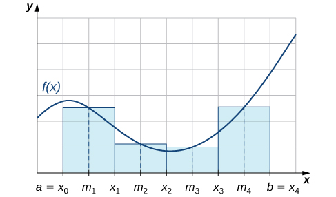
As we can see in Figure \(\PageIndex{1}\), if \( f(x) \geq 0\) over \( [a,b]\), then \(\displaystyle \sum^n_{i=1}f(m_i) \Delta x\) corresponds to the sum of the areas of rectangles approximating the area between the graph of \( f(x)\) and the \(x\)-axis over \([a,b]\). The graph shows the rectangles corresponding to \(M_4\) for a nonnegative function over a closed interval \([a,b]\).
If we are lucky enough to know the exact value of a definite integral, then we can define the absolute error of an estimation as follows:
The absolute error, \( E_* \), of a numerical approximation, \( A \), to the true value of the quantity, \( T \), is defined to be
\[ E_* = |T - A|. \nonumber \]
The notation "\( * \)" is reserved for the method being used. For example, the absolute error if using the Midpoint Rule with \( n = 10 \) to approximate the value of a definite integral is
\[ E_M = \left| T - M_{10} \right|. \nonumber \]
Use the Midpoint Rule to estimate
\[ \int ^1_0x^2\,dx \nonumber \]
using four subintervals. Compare the result with the actual value of this integral.
Solution
Each subinterval has length \( \Delta x=\frac{1−0}{4}=\frac{1}{4}\). Therefore, the subintervals consist of
\[\left[0,\dfrac{1}{4}\right], \, \left[\dfrac{1}{4},\dfrac{1}{2}\right], \, \left[\dfrac{1}{2},\dfrac{3}{4}\right], \, \text{and} \, \left[\dfrac{3}{4},1\right].\nonumber \]
The midpoints of these subintervals are \(\left\{\frac{1}{8},\,\frac{3}{8},\,\frac{5}{8},\, \frac{7}{8}\right\}\). Thus,
\[\begin{array}{rcl}
M_4 & = & \dfrac{1}{4}\cdot f\left(\dfrac{1}{8}\right)+\dfrac{1}{4}\cdot f\left(\dfrac{3}{8}\right)+\dfrac{1}{4}\cdot f\left(\dfrac{5}{8}\right)+\dfrac{1}{4}\cdot f\left(\dfrac{7}{8}\right) \\
& = & \dfrac{1}{4} \cdot \dfrac{1}{64}+\dfrac{1}{4} \cdot \dfrac{9}{64}+\dfrac{1}{4} \cdot \dfrac{25}{64}+\dfrac{1}{4} \cdot \dfrac{49}{64}\\
& = & \dfrac{21}{64} \\
& = & 0.328125. \\
\end{array} \nonumber \]
Since the true value of this definite integral is
\[ T = \int ^1_0x^2\,dx = \dfrac{1}{3},\nonumber \]
the absolute error in this approximation is
\[ E_M = \left| T - M_4\right| = \left| \dfrac{1}{3} − \dfrac{21}{64}\right| = \dfrac{1}{192} \approx 0.0052, \nonumber \]
and we see that the Midpoint Rule produces an estimate that is somewhat close to the actual value of the definite integral.
Use \(M_6\) to estimate the length of the curve
\[y=\dfrac{1}{2}x^2, \nonumber \]
on \([1,4]\).
Solution
The length of \(y=\frac{1}{2}x^2\) on \([1,4]\) is
\[s = \int ^4_1 \sqrt{1+\left(\frac{dy}{dx}\right)^2}\,dx.\nonumber \]
Since \(\dfrac{dy}{dx} = x\), this integral becomes \(\displaystyle \int ^4_1\sqrt{1+x^2}\,dx.\)
If \([1,4]\) is divided into six subintervals, then each subinterval has length \( \Delta x=\frac{4−1}{6}=\frac{1}{2}\) and the midpoints of the subintervals are \(\left\{\frac{5}{4},\frac{7}{4},\frac{9}{4},\frac{11}{4},\frac{13}{4},\frac{15}{4}\right\}\). If we set \(f(x)=\sqrt{1+x^2}\), we get
\[\begin{array}{rcl}
M_6 & = & \dfrac{1}{2}\cdot f\left(\dfrac{5}{4}\right)+\dfrac{1}{2}\cdot f\left(\dfrac{7}{4}\right)+\dfrac{1}{2}\cdot f\left(\dfrac{9}{4}\right)+\dfrac{1}{2}\cdot f\left(\dfrac{11}{4}\right)+\dfrac{1}{2}\cdot f\left(\dfrac{13}{4}\right)+\dfrac{1}{2}\cdot f\left(\dfrac{15}{4}\right) \\
& \approx & \dfrac{1}{2}(1.6008+2.0156+2.4622+2.9262+3.4004+3.8810) \\
& = & 8.1431 \, \text{ units}. \\
\end{array} \nonumber \]
Use \( M_2 \) to estimate
\[ \int ^2_1\frac{1}{x}\,dx. \nonumber \]
- Hint
-
\( \Delta x=\frac{1}{2}, \quad m_1=\frac{5}{4},\quad \text{and} \quad m_2=\frac{7}{4}.\)
- Answer
-
\(\dfrac{24}{35}\approx 0.685714\)
The Trapezoidal Rule
We can also approximate the value of a definite integral by using trapezoids rather than rectangles (see Figure \(\PageIndex{2}\)).
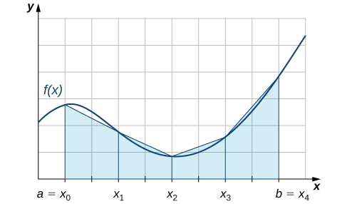
The Trapezoidal Rule for estimating definite integrals uses trapezoids rather than rectangles to approximate the area under a curve. To gain insight into the final form of the rule, consider the trapezoids shown in Figure \(\PageIndex{2}\). We assume that the length of each subinterval is given by \( \Delta x\). First, recall that the area of a trapezoid with a height of \(h\) and bases of length \(b_1\) and \(b_2\) is given by
\[\text{Area}=\frac{1}{2}h(b_1+b_2). \nonumber \]
We see that the first trapezoid has a "height" \( \Delta x\) and parallel "bases" of length \( f(x_0)\) and \( f(x_1)\). Thus, the area of the first trapezoid in Figure \(\PageIndex{2}\) is
\[ \dfrac{1}{2} \Delta x \left(f(x_0)+f(x_1)\right).\nonumber \]
The areas of the remaining three trapezoids are
\[ \dfrac{1}{2} \Delta x \left((f(x_1)+f(x_2)\right),\, \dfrac{1}{2} \Delta x \left(f(x_2)+f(x_3)\right), \text{ and } \dfrac{1}{2} \Delta x \left(f(x_3)+f(x_4)\right). \nonumber \]
Consequently,
\[ \int ^b_af(x)\,dx \approx \dfrac{1}{2} \Delta x \left(f(x_0)+f(x_1)\right)+\dfrac{1}{2} \Delta x \left(f(x_1)+f(x_2)\right) + \dfrac{1}{2} \Delta x \left(f(x_2) + f(x_3)\right) + \dfrac{1}{2} \Delta x\left(f(x_3)+f(x_4)\right).\nonumber \]
After taking out a common factor of \(\frac{1}{2} \Delta x\) and combining like terms, we have
\[ \int ^b_af(x)\,dx \approx \dfrac{\Delta x}{2}\left[f(x_0)+2 f(x_1)+2 f(x_2)+2 f(x_3)+f(x_4)\right].\nonumber \]
Generalizing, we formally state the following rule.
Let \(f(x)\) be continuous over \([a,b]\), \(n\) be a positive integer, and \( \Delta x=\frac{b−a}{n}\). If \( [a,b]\) is divided into \(n\) subintervals, each of length \( \Delta x\), with endpoints at \( P=\{x_0,x_1,x_2, \ldots ,x_n\}\), set
\[T_n=\dfrac{ \Delta x}{2}\left[f(x_0)+2 f(x_1) + 2 f(x_2) + \cdots + 2 f(x_{n−1}) + f(x_n)\right]. \nonumber \]
Then,
\[ \lim_{n \to \infty}T_n = \int ^b_af(x)\,dx. \nonumber \]
Before continuing, let’s make a few observations about the Trapezoidal Rule. First of all, it is useful to note that
\[T_n=\dfrac{1}{2}(L_n+R_n), \text{ where } L_n = \sum_{i=1}^nf(x_{i−1}) \Delta x \text{ and } R_n=\sum_{i=1}^nf(x_i) \Delta x. \nonumber \]
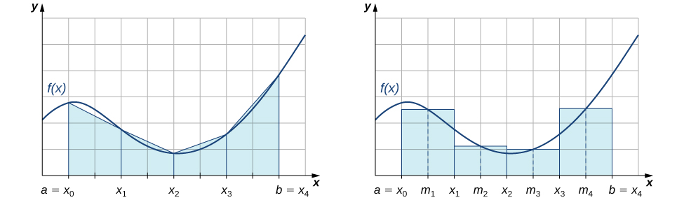
That is, the Trapezoidal Rule is the average of the Left Endpoint Approximation, \(L_n\), and the Right Endpoint Approximation, \(R_n\). In addition, a careful examination of Figure \(\PageIndex{3}\) (see below) leads us to make the following observations about using the Trapezoidal Rules and Midpoint Rules to estimate the definite integral of a nonnegative function. The Trapezoidal Rule tends to overestimate the value of a definite integral systematically over intervals where the function is concave up and to underestimate the value of a definite integral systematically over intervals where the function is concave down. On the other hand, the Midpoint Rule tends to average out these errors somewhat by partially overestimating and partially underestimating the value of the definite integral over these same types of intervals. This leads us to hypothesize that, in general, the Midpoint Rule tends to be more accurate than the Trapezoidal Rule.
Use the Trapezoidal Rule to estimate
\[ \int ^1_0x^2\,dx \nonumber \]
using four subintervals.
Solution
The endpoints of the subintervals consist of elements of the set \(P=\left\{0,\frac{1}{4},\, \frac{1}{2},\, \frac{3}{4},1\right\}\) and \( \Delta x=\frac{1−0}{4}=\frac{1}{4}.\) Thus,
\[\begin{array}{rcl}
\displaystyle \int^1_0 x^2 \, dx & \approx & \dfrac{1}{2} \cdot \dfrac{1}{4} \left[f(0)+2 f\left(\dfrac{1}{4}\right)+2 f\left(\dfrac{1}{2}\right)+2 f\left(\dfrac{3}{4}\right)+f(1)\right] \\
& = & \dfrac{1}{8}\left(0+2 \cdot \dfrac{1}{16}+2 \cdot \dfrac{1}{4}+2 \cdot \dfrac{9}{16}+1\right) \\
& = & \dfrac{11}{32} \\
& = & 0.34375 \\
\end{array} \nonumber \]
Use \( T_2 \) to estimate
\[ \int ^2_1\frac{1}{x}\,dx. \nonumber \]
- Hint
-
Set \( \Delta x=\frac{1}{2}.\) The endpoints of the subintervals are the elements of the set \(P=\left\{1,\frac{3}{2},2\right\}.\)
- Answer
-
\(\dfrac{17}{24} \approx 0.708333\)
Absolute and Relative Error
An important aspect of using these numerical approximation rules consists of calculating the error in using them for estimating the value of a definite integral. As was mentioned earlier, the absolute error for a method is given by
\[ E_* = \left| T - A \right|. \nonumber \]
Another important measure is the relative error of an approximation.
The relative error of an approximation is the error as a percentage of the actual value and is given by
\[\left| \dfrac{T − A_*}{T}\right| \cdot 100\% = \dfrac{E_*}{|T|} \cdot 100\%. \nonumber \]
Calculate the relative error in the estimate of \(\displaystyle \int ^1_0x^2\,dx\) using the Midpoint Rule, found in Example \(\PageIndex{1}\).
Solution
We computed the absolute error to be \( E_M \approx 0.0052\). Therefore, the relative error is
\[ \left| \dfrac{T - M_4}{T} \right| = \dfrac{E_M}{|T|} = \dfrac{1/192}{1/3}=\dfrac{1}{64} \approx 0.015625 \approx 1.6\%.\nonumber \]
Calculate the absolute and relative error in the estimate of \(\displaystyle \int ^1_0x^2\,dx\) using the Trapezoidal Rule, found in Example \(\PageIndex{3}\).
Solution
The true value is \(\displaystyle \int ^1_0x^2\,dx=\frac{1}{3}\), and our estimate from the example is \(T_4=\frac{11}{32}\). Thus, the absolute error is given by
\[ E_T = \left| T - T_4 \right| = \left|\dfrac{1}{3}−\dfrac{11}{32}\right| = \dfrac{1}{96} \approx 0.0104. \nonumber \]
The relative error is given by
\[\left| \dfrac{T − T_4}{T}\right| = \dfrac{E_T}{|T|} = \dfrac{1/96}{1/3} = 0.03125 \approx 3.1\%.\nonumber \]
In an earlier checkpoint, we estimated \(\displaystyle \int ^2_1\frac{1}{x}\,dx\) to be \(\frac{24}{35}\) using \(M_2\). The actual value of this integral is \(\ln 2\). Using \(\frac{24}{35} \approx 0.6857\) and \(\ln 2 \approx 0.6931\), calculate the absolute error and the relative error.
- Hint
-
Use the previous examples as a guide.
- Answer
-
The absolute error is \(\approx 0.0074\), and the relative error is \(\approx 1.1\%\).
Error Bounds on the Midpoint and Trapezoidal Rules
In the two previous examples, we were able to compare our estimate of an integral with the actual value of the integral; however, we do not typically have this luxury. In general, if we are approximating an integral, we are doing so because we cannot compute the exact value of the integral itself easily. Therefore, it is often helpful to be able to determine an upper bound for the error in an approximation of an integral. The following theorem provides error bounds for the Midpoint and Trapezoidal Rules. The theorem is stated without proof.1
Let \(f(x)\) be a continuous function over \([a,b]\), where \(f^{\prime\prime}(x)\) exists over this same interval interval. If \(M\) is the maximum value of \(\left|f^{\prime\prime}(x)\right|\) over \([a,b]\), then the upper bounds for the error in using \(M_n\) and \(T_n\) to estimate \(\displaystyle \int ^b_af(x)\,dx\) are
\[E_M \leq \dfrac{M(b−a)^3}{24n^2} \label{MidError} \]
and
\[E_T \leq \frac{M(b−a)^3}{12n^2}. \label{TrapError} \]
We can use these bounds to determine the value of \(n\) necessary to guarantee that the error in an estimate is less than a specified value.
What value of \(n\) should be used to guarantee that an estimate of
\[ \int ^1_0e^{x^2}\,dx \nonumber \]
is accurate to within \(0.01\) if we use the Midpoint Rule?
Solution
We begin by determining the value of \(M\), the maximum value of \( \left|f^{\prime\prime}(x)\right|\) over \( [0,1]\) for \( f(x)=e^{x^2}\).
Since \( f^{\prime}(x)=2xe^{x^2},\) we have
\[ f^{\prime\prime}(x)=2e^{x^2}+4x^2e^{x^2}.\nonumber \]
Thus,
\[ \left|f^{\prime\prime}(x)\right| = 2e^{x^2}(1+2x^2) \leq 2 \cdot e \cdot 3 = 6e.\nonumber \]
From the error-bound Equation \(\ref{MidError}\), we have
\[ E_M \leq \dfrac{M(b−a)^3}{24n^2} \leq \dfrac{6e(1−0)^3}{24n^2}=\dfrac{6e}{24n^2}.\nonumber \]
Now we solve the following inequality for \(n\):
\[\frac{6e}{24n^2} \leq 0.01.\nonumber \]
Thus, \(n \geq \sqrt{\frac{600e}{24}} \approx 8.24\). Since \(n\) must be an integer satisfying this inequality, a choice of \(n=9\) would guarantee that
\[ E_M = \left|T - M_n \right| = \left| \int ^1_0e^{x^2}\,dx − M_n \right| \lt 0.01.\nonumber \]
Analysis
We might have been tempted to round \(8.24\) down and choose \(n=8\), but this would be incorrect because we must have an integer greater than or equal to \(8.24\). We need to keep in mind that the error estimates provide an upper bound only for the error. The actual estimate may, in fact, be a much better approximation than is indicated by the error bound.
Use Equation \(\ref{MidError}\) to find an upper bound for the error in using \(M_4\) to estimate \(\displaystyle \int ^1_0x^2\,dx.\)
- Hint
-
\(f^{\prime\prime}(x)=2,\) so \(M=2.\)
- Answer
-
\(\dfrac{1}{192}\)
1 The exploration of numerical methods, their error bounds, and the trade off between the accuracy of the method and its computational expense is the realm of a subfield of Mathematics called Numerical Analysis. If you are intrigued by how such methods (and their errors) are developed, I recommend taking a series of upper division courses in Numerical Analysis.
Simpson's Rule
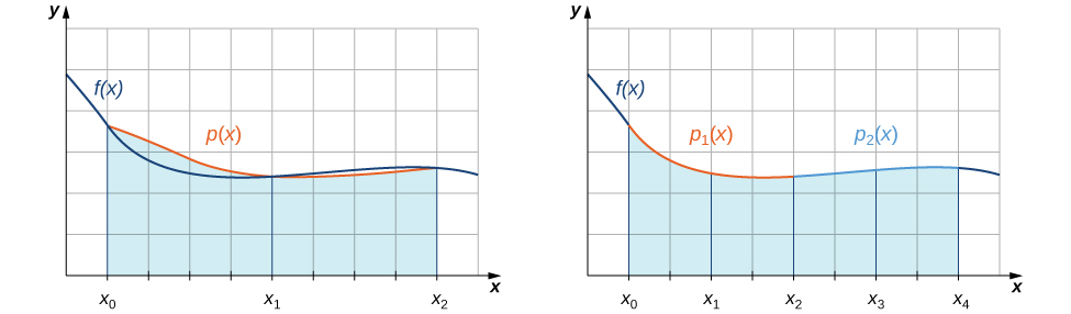
With the Midpoint Rule, we estimated areas of regions under curves by using rectangles. In a sense, we approximated the curve with piecewise constant functions. With the Trapezoidal Rule, we approximated the curve by using piecewise linear functions. What if we were, instead, to approximate a curve using piecewise quadratic functions? With Simpson's Rule, we do just this. We partition the interval into an even number of subintervals, each of equal width. Over the first pair of subintervals we approximate \(\displaystyle \int ^{x_2}_{x_0} f(x)\,dx\) with \(\displaystyle \int ^{x_2}_{x_0}p(x)\,dx\), where \(p(x)=Ax^2+Bx+C\) is the quadratic function passing through \((x_0,f(x_0)), \,(x_1,f(x_1)),\) and \((x_2,f(x_2))\) (Figure \(\PageIndex{4}\)). Over the next pair of subintervals we approximate \(\displaystyle \int ^{x_4}_{x_2}f(x)\,dx\) with the integral of another quadratic function passing through \( (x_2,f(x_2)), \,(x_3,f(x_3)),\) and \((x_4,f(x_4)).\) This process is continued with each successive pair of subintervals.
To understand the formula that we obtain for Simpson's Rule, we begin by deriving a formula for this approximation over the first two subintervals. As we go through the derivation, we need to keep in mind the following relationships:
\[ \begin{array}{rclcl}
f(x_0) & = & p(x_0) & = & Ax_0^2+Bx_0+C \\
f(x_1) & = & p(x_1) & = & Ax_1^2+Bx_1+C \\
f(x_2) & = & p(x_2) & = & Ax_2^2+Bx_2+C \\
\end{array} \nonumber \]
\[ x_2 − x_0 = 2 \Delta x, \text{ where } \Delta x \text{ is the length of a subinterval,} \nonumber \]
\[ \text{and } x_2+x_0=2x_1, \text{ since } x_1=\dfrac{(x_2+x_0)}{2}. \nonumber \]
Thus,
\[\begin{array}{rclr}
\displaystyle \int ^{x_2}_{x_0}f(x)\,dx & \approx & \displaystyle \int ^{x_2}_{x_0}p(x)\,dx & \\
& = & \displaystyle \int^{x_2}_{x_0}(Ax^2+Bx+C)\,dx & \\
& = & \left(\dfrac{A}{3}x^3+\dfrac{B}{2}x^2+Cx\right)\bigg|^{x_2}_{x_0} & \\
& = & \dfrac{A}{3}(x_2^3−x_0^3)+\dfrac{B}{2}(x_2^2−x_0^2)+C(x_2−x_0) & \\
& = & \dfrac{A}{3}(x_2−x_0)(x_2^2+x_2x_0+x_0^2)+\dfrac{B}{2}(x_2−x_0)(x_2+x_0)+C(x_2−x_0) & \left( \text{Factor.} \right)\\
& = & \dfrac{x_2−x_0}{6} \left( 2A(x_2^2+x_2x_0+x_0^2)+3B(x_2+x_0)+6C \right) & \left( \text{Factor out } \frac{x_2−x_0}{6}. \right) \\
& = & \dfrac{\Delta x}{3} \left[ (Ax_2^2+Bx_2+C)+(Ax_0^2+Bx_0+C)+A(x_2^2+2x_2x_0+x_0^2)+2B(x_2+x_0)+4C \right] & \bigg( \text{Rearrange terms.} \\
& & & \text{Note: } \Delta x = \dfrac{x_2−x_0}{2} \bigg) \\
& = & \dfrac{\Delta x}{3} \left[ f(x_2)+f(x_0)+A(x_2+x_0)^2+2B(x_2+x_0)+4C \right] & \bigg( \text{Factor and substitute:} \\
& & & f(x_2) = Ax_2^2+Bx_2+C \\
& & & \text{and } f(x_0)=Ax_0^2+Bx_0+C. \bigg) \\
& = & \dfrac{\Delta x}{3}\left[ f(x_2)+f(x_0)+A(2x_1)^2+2B(2x_1)+4C\right] & \bigg( \text{Substitute }x_2+x_0=2x_1. \\
& & & \text{Note: } x_1 = \dfrac{x_2+x_0}{2} \text{ is the midpoint.} \bigg) \\
& = & \dfrac{\Delta x}{3}\left(f(x_2)+4f(x_1)+f(x_0)\right). & \bigg(\text{Expand and substitute} \\
& & & f(x_1)=Ax_1^2+Bx_1+C.\bigg) \\
\end{array} \nonumber \]
If we approximate \(\displaystyle \int ^{x_4}_{x_2}f(x)\,dx\) using the same method, we see that we have
\[ \int ^{x_4}_{x_2}f(x)\,dx \approx \dfrac{ \Delta x}{3}(f(x_4)+4\,f(x_3)+f(x_2)).\nonumber \]
Combining these two approximations, we get
\[ \int ^{x_4}_{x_0}f(x)\,dx \approx \dfrac{ \Delta x}{3}(f(x_0)+4\,f(x_1)+2\,f(x_2)+4\,f(x_3)+f(x_4)).\nonumber \]
The pattern continues as we add pairs of subintervals to our approximation. The general rule may be stated as follows.
Assume that \(f(x)\) is continuous over \([a,b]\). Let \(n\) be a positive even integer and \( \Delta x=\frac{b−a}{n}\). Let \([a,b]\) be divided into \(n\) subintervals, each of length \( \Delta x\), with endpoints at \(P=\{x_0,x_1,x_2, \ldots ,x_n\}\). Set
\[S_n = \dfrac{\Delta x}{3}\left[f(x_0)+4f(x_1)+2f(x_2)+4f(x_3)+2f(x_4) + \cdots +2f(x_{n−2})+4f(x_{n−1})+f(x_n)\right]. \nonumber \]
Then,
\[\lim_{n \to \infty }S_n= \int ^b_af(x)\,dx.\nonumber \]
Just as the Trapezoidal Rule is the average of the Left Endpoint and Right Endpoint Approximations for estimating definite integrals, Simpson's Rule may be obtained from the Midpoint and Trapezoidal Rules by using a weighted average. It can be shown that \(S_{2n} = \left(\frac{2}{3}\right)M_n+\left(\frac{1}{3}\right)T_n\).
It is also possible to put a bound on the error when using Simpson's Rule to approximate a definite integral. The bound in the error is given by the following rule:
Let \(f(x)\) be a continuous function over \([a,b]\) having a fourth derivative, \( f^{(4)}(x)\), over this interval. If \(M\) is the maximum value of \(\left|f^{(4)}(x)\right|\) over \([a,b]\), then the upper bound for the error in using \(S_n\) to estimate \(\displaystyle \int ^b_af(x)\,dx\) is given by
\[E_S \leq \frac{M(b−a)^5}{180n^4}. \nonumber \]
Use \(S_2\) to approximate
\[ \int ^1_0x^3\,dx. \nonumber \]
Estimate a bound for the error in \(S_2\).
Solution
Since \([0,1]\) is divided into two intervals, each subinterval has length \( \Delta x=\frac{1−0}{2}=\frac{1}{2}\). The endpoints of these subintervals are \(\left\{0,\frac{1}{2},1\right\}\). If we set \(f(x)=x^3,\) then
\[S_2 = \dfrac{1/2}{3} \left( f(0)+4 f\left(\dfrac{1}{2}\right)+f(1) \right) = \dfrac{1}{6} \left(0+4 \cdot \dfrac{1}{8}+1 \right) = \dfrac{1}{4}.\nonumber \]
Since \( f^{(4)}(x)=0\) and consequently \(M=0,\) we see that
\[ E_S \leq \dfrac{0(1)^5}{180 \cdot 2^4} = 0. \nonumber \]
This bound indicates that the value obtained through Simpson's Rule is exact. A quick check will verify that, in fact, \(\displaystyle \int ^1_0x^3\,dx=\frac{1}{4}\).
Use \(S_6\) to estimate the length of the curve
\[y=\frac{1}{2}x^2 \nonumber \]
over \([1,4]\)
Solution
The length of \(y=\frac{1}{2}x^2\) over \([1,4]\) is \(\displaystyle \int ^4_1\sqrt{1+x^2}\,dx\). If we divide \([1,4]\) into six subintervals, then each subinterval has length \( \Delta x=\frac{4−1}{6}=\frac{1}{2}\), and the endpoints of the subintervals are \( \left\{1,\frac{3}{2},2,\frac{5}{2},3,\frac{7}{2},4\right\}.\) Setting \( f(x)=\sqrt{1+x^2}\),
\[ S_6 = \dfrac{1/2}{3} \left(f(1)+4f\left(\dfrac{3}{2}\right)+2f(2)+4f\left(\dfrac{5}{2}\right)+2f(3)+4f\left(\dfrac{7}{2}\right)+f(4)\right).\nonumber \]
After substituting, we have
\[S_6=\dfrac{1}{6} \left(1.4142+4 \cdot 1.80278+2 \cdot 2.23607+4 \cdot 2.69258+2 \cdot 3.16228+4 \cdot 3.64005+4.12311 \right) \approx 8.14594\,\text{units}. \nonumber \]
Use \(S_2\) to estimate
\[ \int ^2_1\frac{1}{x}\,dx. \nonumber \]
- Hint
-
\[S_2=\frac{1}{3} \Delta x\left(f(x_0)+4f(x_1)+f(x_2)\right) \nonumber \]
- Answer
-
\(\frac{25}{36} \approx 0.694444\)
Key Concepts
- We can use numerical integration to estimate the values of definite integrals when a closed form of the integral is difficult to find or when an approximate value only of the definite integral is needed.
- The most commonly used techniques for numerical integration are the Midpoint Rule, Trapezoidal Rule, and Simpson's Rule.
- The Midpoint Rule approximates the definite integral using rectangular regions whereas the Trapezoidal Rule approximates the definite integral using trapezoidal approximations.
- Simpson's Rule approximates the definite integral by first approximating the original function using piecewise quadratic functions.
Key Equations
- Midpoint Rule
\(\displaystyle M_n=\sum^n_{i=1}f(m_i) \Delta x\)
- Trapezoidal Rule
\(T_n=\frac{ \Delta x}{2}\Big[f(x_0)+2\,f(x_1)+2\,f(x_2)+ \cdots +2\,f(x_{n−1})+f(x_n)\Big]\)
- Simpson's Rule
\(S_n=\frac{ \Delta x}{3}\Big[f(x_0)+4\,f(x_1)+2\,f(x_2)+4\,f(x_3)+2\,f(x_4)+4\,f(x_5)+ \cdots +2\,f(x_{n−2})+4\,f(x_{n−1})+f(x_n)\Big]\)
- Error bound for Midpoint Rule
Error in \(M_n \leq \dfrac{M(b−a)^3}{24n^2}\), where \(M\) is the maximum value of \(|f''(x)|\) over \([a,b]\).
- Error bound for Trapezoidal Rule
Error in \(T_n \leq \dfrac{M(b−a)^3}{12n^2}\), where \(M\) is the maximum value of \(|f''(x)|\) over \([a,b]\).
- Error bound for Simpson's Rule
Error in \(S_n \leq \dfrac{M(b−a)^5}{180n^4}\), where \(M\) is the maximum value of \(∣f^{(4)}(x)∣\) over \([a,b]\).
Glossary
- absolute error
- if \(B\) is an estimate of some quantity having an actual value of \(A\), then the absolute error is given by \( |A−B|\)
- Midpoint Rule
- a rule that uses a Riemann sum of the form \(\displaystyle M_n=\sum^n_{i=1}f(m_i) \Delta x\), where \( m_i\) is the midpoint of the \(i^{\text{th}}\) subinterval to approximate \(\displaystyle \int ^b_af(x)\,dx\)
- numerical integration
- the variety of numerical methods used to estimate the value of a definite integral, including the Midpoint Rule, Trapezoidal Rule, and Simpson's Rule
- relative error
- error as a percentage of the actual value, given by \[\text{relative error}=\left|\frac{A−B}{A}\right| \cdot 100\%\nonumber \]
- Simpson's Rule
- a rule that approximates \(\displaystyle \int ^b_af(x)\,dx\) using the area under a piecewise quadratic function.
The approximation \(S_n\) to \(\displaystyle \int ^b_af(x)\,dx\) is given by \[S_n=\frac{ \Delta x}{3}\big(f(x_0)+4\,f(x_1)+2\,f(x_2)+4\,f(x_3)+2\,f(x_4)+ \cdots +2\,f(x_{n−2})+4\,f(x_{n−1})+f(x_n)\big).\nonumber \]
- Trapezoidal Rule
- a rule that approximates \(\displaystyle \int ^b_af(x)\,dx\) using the area of trapezoids.
The approximation \(T_n\) to \(\displaystyle \int ^b_af(x)\,dx\) is given by \[T_n=\frac{ \Delta x}{2}\big(f(x_0)+2\, f(x_1)+2\, f(x_2)+ \cdots +2\, f(x_{n−1})+f(x_n)\big).\nonumber \]
Review Topics (from previous courses)
Arithmetic
Algebra
Geometry
- area of a trapezoid