1.3: Direction Fields

It’s impossible to find explicit formulas for solutions of some differential equations. Even if there are such formulas, they may be so complicated that they’re useless. In this case we may resort to graphical or numerical methods to get some idea of how the solutions of the given equation behave.

In Section 1.2 we talked about the existence of solutions of a first order equation \[\label{eq:1.3.1} y'=f(x,y).\]

In this section we’ll simply assume that Equation \ref{eq:1.3.1} has solutions and discuss a graphical method for approximating them. In Chapter 3 we discuss numerical methods for obtaining approximate solutions of Equation \ref{eq:1.3.1}. Recall that a solution of Equation \ref{eq:1.3.1} is a function \(y=y(x)\) such that

\[y'(x)=f(x,y(x))\nonumber \]

for all values of \(x\) in some interval, and an integral curve is either the graph of a solution or is made up of segments that are graphs of solutions. Therefore, not being able to solve Equation \ref{eq:1.3.1} is equivalent to not knowing the equations of integral curves of Equation \ref{eq:1.3.1}. However, it is easy to calculate the slopes of these curves. To be specific, the slope of an integral curve of Equation \ref{eq:1.3.1} through a given point \((x_0,y_0)\) is given by the number \(f(x_0,y_0)\). This is the basis of the method of direction fields.

If \(f\) is defined on a set \(R\), we can construct a direction field for Equation \ref{eq:1.3.1} in \(R\) by drawing a short line segment through each point \((x,y)\) in \(R\) with slope \(f(x,y)\). Of course, as a practical matter, we can’t actually draw line segments through every point in \(R\); rather, we must select a finite set of points in \(R\). For example, suppose \(f\) is defined on the closed rectangular region \[R:\{a\le x\le b, c\le y\le d\}.\nonumber \]

Let \[a= x_0< x_1< \cdots< x_m=b\nonumber \] be equally spaced points in \([a,b]\) and \[c=y_{0}<y_{1}<\cdots< y_{n}=d\nonumber \] form a rectangular grid (Figure 1.3.1 ). Through each point in the grid we draw a short line segment with slope \(f(x_i,y_j)\). The result is an approximation to a direction field for Equation \ref{eq:1.3.1} in \(R\). If the grid points are sufficiently numerous and close together, we can draw approximate integral curves of Equation \ref{eq:1.3.1} by drawing curves through points in the grid tangent to the line segments associated with the points in the grid.

Figure 1.3.1 : A rectangular grid

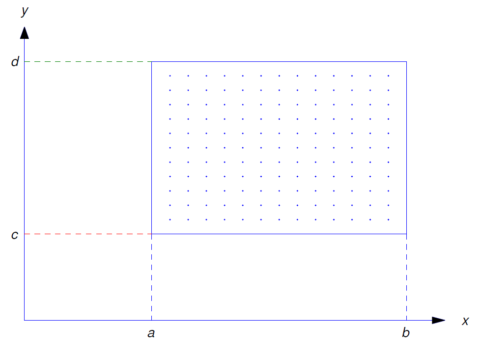
Unfortunately, approximating a direction field and graphing integral curves in this way is too tedious to be done effectively by hand. However, there is software for doing this. As you’ll see, the combination of direction fields and integral curves gives useful insights into the behavior of the solutions of the differential equation even if we can’t obtain exact solutions.

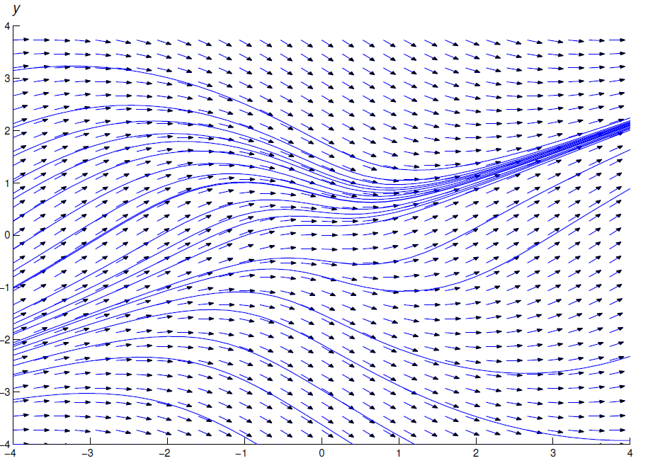
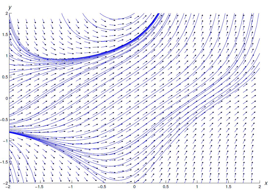
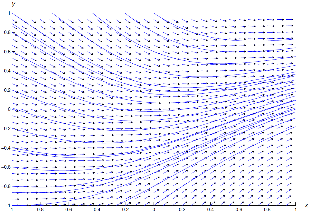
We’ll study numerical methods for solving a single first order equation Equation \ref{eq:1.3.1} in Chapter 3. These methods can be used to plot solution curves of Equation \ref{eq:1.3.1} in a rectangular region \(R\) if \(f\) is continuous on \(R\). Figures 1.3.2 , 1.3.3 , and 1.3.4 show direction fields and solution curves for the differential equations:

• \(y'=\frac{x^2-y^2}{1+x^2+y^2}\),
• \(y'=1+xy^2\), and
• \(y'=\frac{x-y}{1+x^2}\).

which are all of the form Equation \ref{eq:1.3.1} with \(f\) continuous for all \((x,y)\).

Figure 1.3.2 : A direction and integral curves for \(y'= {\frac{x^2-y^2}{1+x^2+y^2}}\).

Figure 1.3.3 : A direction and integral curves for \(y'= 1 + xy^2\).

Figure 1.3.4 : A direction and integral curves for \(y'= {\frac{x-y}{1+x^2}}\).

The methods of Chapter 3 will not work for the equation \[\label{eq:1.3.2} y'=-x/y\]

if \(R\) contains part of the \(x\)-axis, since \(f(x,y)=-x/y\) is undefined when \(y=0\). Similarly, they will not work for the equation

\[\label{eq:1.3.3} y'={x^2\over1-x^2-y^2}\]

if \(R\) contains any part of the unit circle \(x^2+y^2=1\), because the right side of Equation \ref{eq:1.3.3} is undefined if \(x^2+y^2=1\). However, Equation \ref{eq:1.3.2} and Equation \ref{eq:1.3.3} can written as

\[\label{eq:1.3.4} y'={A(x,y)\over B(x,y)}\]

where \(A\) and \(B\) are continuous on any rectangle \(R\). Because of this, some differential equation software is based on numerically solving pairs of equations of the form

\[\label{eq:1.3.5} {dx\over dt}=B(x,y),\quad {dy\over dt}=A(x,y)\]

where \(x\) and \(y\) are regarded as functions of a parameter \(t\). If \(x=x(t)\) and \(y=y(t)\) satisfy these equations, then

\[y'={dy\over dx}={dy\over dt}\left/{dx\over dt}\right.={A(x,y)\over B(x,y)},\nonumber\]

so \(y=y(x)\) satisfies Equation \ref{eq:1.3.4}.

Equations \ref{eq:1.3.2} and \ref{eq:1.3.3} can be reformulated as in Equation \ref{eq:1.3.4} with \[{dx\over dt}=-y,\quad {dy\over dt}=x\nonumber\]

and

\[{dx\over dt}=1-x^2-y^2,\quad {dy\over dt}=x^2,\nonumber \]

respectively. Even if \(f\) is continuous and otherwise “nice” throughout \(R\), your software may require you to reformulate the equation \(y'=f(x,y)\) as

\[{dx\over dt}=1,\quad {dy\over dt}=f(x,y),\nonumber \]

which is of the form Equation \ref{eq:1.3.5} with \(A(x,y)=f(x,y)\) and \(B(x,y)=1\).

Figure 1.3.5 shows a direction field and some integral curves for Equation \ref{eq:1.3.2}. As we saw in Example 1.1.1 and will verify again in Section 2.1, the integral curves of Equation \ref{eq:1.3.2} are circles centered at the origin.

Figure 1.3.5 : A direction field and integral curves for \(y'=- {x\over y}\)

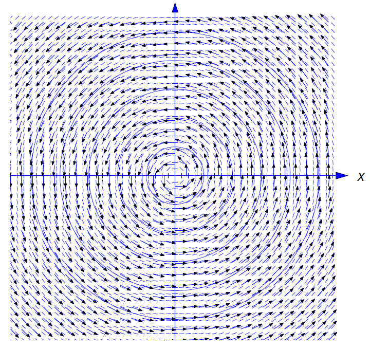
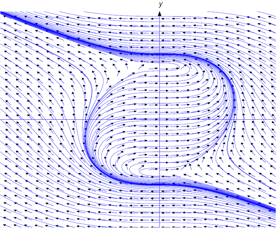
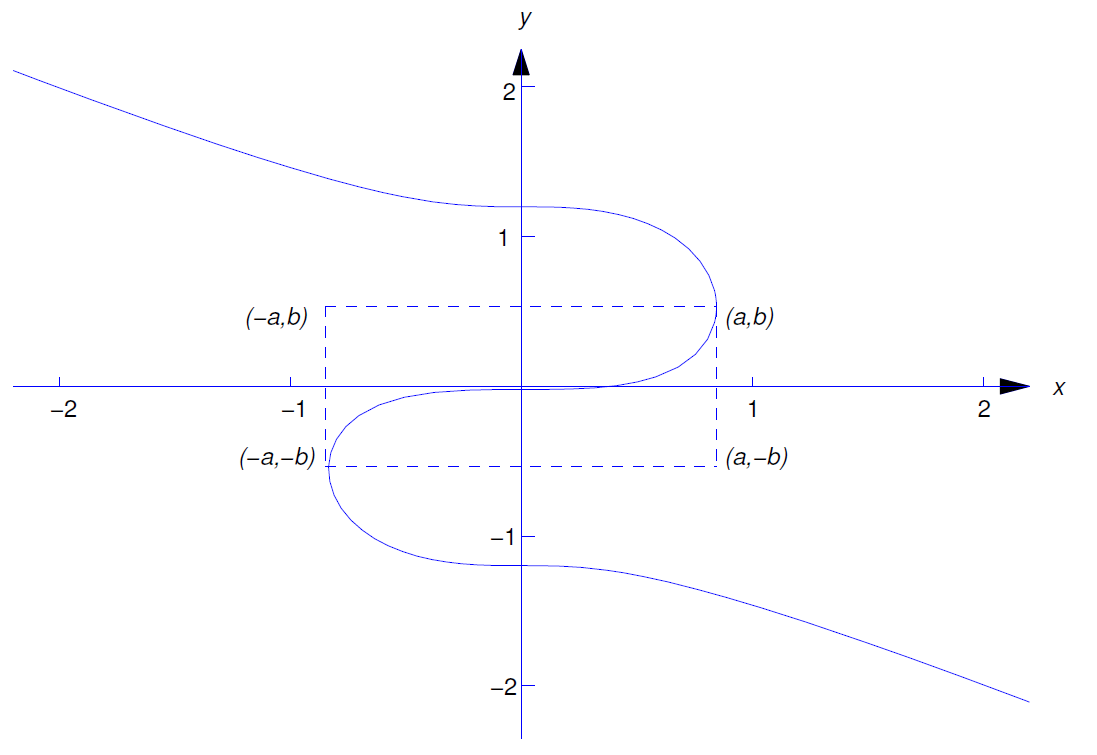
Figure 1.3.6 shows a direction field and some integral curves for Equation \ref{eq:1.3.3}. The integral curves near the top and bottom are solution curves. However, the integral curves near the middle are more complicated. For example, Figure 1.3.7 shows the integral curve through the origin. The vertices of the dashed rectangle are on the circle \(x^2+y^2=1\) ( \(a\approx.846\), \(b\approx.533\)), where all integral curves of Equation \ref{eq:1.3.3} have infinite slope. There are three solution curves of Equation \ref{eq:1.3.3} on the integral curve in the figure: the segment above the level \(y=b\) is the graph of a solution on \((-\infty,a)\), the segment below the level \(y=-b\) is the graph of a solution on \((-a,\infty)\), and the segment between these two levels is the graph of a solution on \((-a,a)\).

Figure 1.3.6 : A direction field and integral curves for \(y'= \dfrac{x^2}{1-x^2-y^2}\).

Figure 1.3.7 : A direction field and integral curves for \(y'= \dfrac{x^2}{1-x^2-y^2}\)