2.3: Linear First Order Equations

Definition 2.3.1

A first order differential equation is said to be linear if it can be written in the form

\[\label{eq:2.1.1} y' + p(x)y = f(x).\]

A first order differential equation that cannot be written like this is nonlinear.

Example 2.3.1

The first order equations

\[\begin{aligned} x ^ { 2 } y ^ { \prime } + 3 y & = x ^ { 2 } \\[4pt] x y ^ { \prime } - 8 x ^ { 2 } y & = \sin x \\[4pt] x y ^ { \prime } + ( \ln x ) y & = 0 \\[4pt] y ^ { \prime } & = x ^ { 2 } y - 2 \end{aligned}\]

are not in the form in Equation \ref{eq:2.1.1}, but they are linear, since they can be rewritten as

\[\begin{aligned} y ^ { \prime } + \frac { 3 } { x ^ { 2 } } y & = 1 \\[4pt] y ^ { \prime } - 8 x y & = \frac { \sin x } { x } \\[4pt] y ^ { \prime } + \frac { \ln x } { x } y & = 0 \\[4pt] y ^ { \prime } - x ^ { 2 } y & = - 2 \end{aligned}\]

Example 2.3.2

Here are some nonlinear first order equations:

\[\begin{aligned} x y ^ { \prime } + 3 y ^ { 2 } & = 2 x & \text { (because } y \text { is squared) } \\[4pt] y y ^ { \prime } & = 3 & \text { (because of the product } y y ^ { \prime } ) \\[4pt] y ^ { \prime } + x e ^ { y } & = 12 & \text { (because of } e ^ { y } ) \end{aligned}\]

In the following theorem we discuss how to solve linear differential equations.

Theorem 2.3.1

If \(p\) is continuous on \((a,b),\) then multiplying the differential equation

\[\label{eq:2.1.12} y'+p(x)y=0\]

on \((a,b)\) by

\[e^{\int p(x)\,dx} \nonumber\]

will make the differential equation exact.

Note: we call \(e^{\int p(x)\,dx} \nonumber\) an integrating factor of the differential equation.

Proof

Consider the first order linear equation

\[ y'+p(x)y=0\nonumber\]

Rewriting this in the form

\[M(x,y)\,dx+N(x,y)\,dy=0\nonumber\]

we get

\[p(x)y\,dx+\,dy=0\nonumber\]

If we multiply this by \(e^{\int p(x)\,dx}\) we get

\[e^{\int p(x)\,dx}p(x)y\,dx+e^{\int p(x)\,dx}\,dy=0, \nonumber\]

Note that this is an exact differential equation (verify this) resulting in the following:

\[d[e^{\int p(x)\,dx}y]\,=0, \nonumber\]

Integrating both sides leads to the solution:

\[e^{\int p(x)\,dx}y\,=c, \nonumber\]

or

\[y=ce^{-\int p(x)\,dx}\ \nonumber\]

Note that in this special case the solution is immediately found from the formula given in the last line of the proof.

Example 2.3.3

a. Find the general solution of

\[xy'+y=0.\label{eq:2.1.8}\]

b. Solve the initial value problem

\[xy'+y=0,\quad y(1)=3.\label{eq:2.1.9}\]

Solution a

We rewrite Equation \ref{eq:2.1.8} as

\[\label{eq:2.1.10} y'+{1\over x}y=0,\]

where \(x\) is restricted to either \((-\infty,0)\) or \((0,\infty)\). If \(y\) is a nontrivial solution of Equation \ref{eq:2.1.10}, there must be some open interval I on which \(y\) has no zeros. From the last line of the proof, we can readily find the solution:

\[y=ce^{-\int{1\over x} \,dx} \nonumber\]

which, after integrating and simplifying, leads to the final answer:

\[\label{eq:2.1.11} y={c\over x}\]

We have now shown that every solution of Equation \ref{eq:2.1.10} is given by Equation \ref{eq:2.1.11} for some choice of \(c\). (Even though we assumed that \(y\) was nontrivial to derive Equation \ref{eq:2.1.11}, we can get the trivial solution by setting \(c=0\) in Equation \ref{eq:2.1.11}.) Conversely, any function of the form Equation \ref{eq:2.1.11} is a solution of Equation \ref{eq:2.1.10}, since differentiating Equation \ref{eq:2.1.11} yields

\[y'=-{c\over x^2}, \nonumber\]

and substituting this and Equation \ref{eq:2.1.11} into Equation \ref{eq:2.1.10} yields

\[\begin{aligned} y'+{1\over x}y=-{c\over x^2}+{1\over x}{c\over x}\\[4pt] =-{c\over x^2}+{c\over x^2}=0.\end{aligned}\]

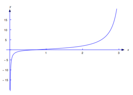
Figure 2.3.2 shows the graphs of some solutions corresponding to various values of \(c\)

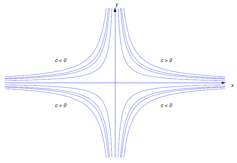
Figure 2.3.2 : Solutions of \(xy'+y=0\) on \((0,\infty)\) and \((-\infty,0)\)

Solution b

Imposing the initial condition \(y(1)=3\) in Equation \ref{eq:2.1.11} yields \(c=3\). Therefore the solution of Equation \ref{eq:2.1.9} is

\[y={3\over x}. \nonumber\]

The interval of validity of this solution is \((0,\infty)\).

General Solution of a Linear First Order Equation

Consider the first order linear equation

\[\label{eq:2.1.4} y'+p(x)y=f(x);\]

Writing this in the form

\[y'=f(x)-p(x)y;\]

note that, if \(p\) and \(f\) are continuous on some open interval \((a,b)\) then (by theorem 1.2.1) there exists a unique solution of the form \(y=y(x,c)\) that involves \(x\) and a parameter \(c\) and has the these properties:

• For each fixed value of \(c\), the resulting function of \(x\) is a solution of Equation \ref{eq:2.1.4} on \((a,b)\).
• If \(y\) is a solution of Equation \ref{eq:2.1.4} on \((a,b)\), then \(y\) can be obtained from the formula by choosing \(c\) appropriately.

\(y=y(x,c)\) is the general solution of Equation \ref{eq:2.1.4}.

When this has been established, it will follow that an equation of the form

\[\label{eq:2.1.5} P_0(x)y'+P_1(x)y=F(x)\]

has a general solution on any open interval \((a,b)\) on which \(P_0\), \(P_1\), and \(F\) are all continuous and \(P_0\) has no zeros, since in this case we can rewrite Equation \ref{eq:2.1.5} in the form Equation \ref{eq:2.1.4} with \(p=P_1/P_0\) and \(f=F/P_0\), which are both continuous on \((a,b)\).

To avoid awkward wording in examples and exercises, we will not specify the interval \((a,b)\) when we ask for the general solution of a specific linear first order equation. Let’s agree that this always means that we want the general solution on every open interval on which \(p\) and \(f\) are continuous if the equation is of the form Equation \ref{eq:2.1.4}, or on which \(P_0\), \(P_1\), and \(F\) are continuous and \(P_0\) has no zeros, if the equation is of the form Equation \ref{eq:2.1.5}. We leave it to you to identify these intervals in specific examples and exercises.

For completeness, we point out that if \(P_0\), \(P_1\), and \(F\) are all continuous on an open interval \((a,b)\), but \(P_0\) does have a zero in \((a,b)\), then Equation \ref{eq:2.1.5} may fail to have a general solution on \((a,b)\) in the sense just defined. Since this isn’t a major point that needs to be developed in depth, we will not discuss it further.

The method for solving

\[\label{eq:2.1.17} y'+p(x)y=f(x)\]

is largely the same in regards to the left hand side of the equation as when \(f(x)\equiv 0\), but we do handle it in a more efficient manner, as the next example illustrates.

Example 2.3.4

Find the general solution of

\[\label{eq:2.1.19} y'+2y=x^3e^{-2x}.\]

Solution

We first find the integrating factor:

\[y=e^{\int 2\,dx}=e^{2x}\nonumber\]

Now multiplying both sides of \ref{eq:2.1.19} by the integrating factor we get

\[e^{2x}y'+2e^{2x}y=x^3.\nonumber\]

Now the left hand side of the equation is exact as we saw when \(f(x)\equiv 0\), but because this isn't the case here we can take a different and better approach. Note that we can write the above as

\[{d\over dx}[e^{2x}y]=x^3.\nonumber\]

Note: the left hand side becomes the derivative of the integrating factor times the dependent variable, which, as we saw earlier, will always be the case. Rewriting this we have

\[{d}[e^{2x}y]=x^3dx.\nonumber\]

Integrating both sides gives us

\[e^{2x}y={x^4\over 4}+c.\nonumber\]

Solving for y we get the general solution of the differential Equation \ref{eq:2.1.19}

\[y={x^4\over 4}e^{-2x}+ce^{-2x}.\nonumber\]

Figure 2.3.3 : A direction field and integral curves for \(y'+2y=x^{2}e^{-2x}\)

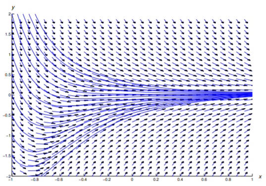
Figure 2.3.3 shows a direction field and some integral curves for Equation \ref{eq:2.1.19}.

Example 2.3.5

a. Find the general solution

\[\label{eq:2.1.29} (\sin x)y'+(\cos x)y=x.\]

b. Solve the initial value problem

\[\label{eq:2.1.30} (\sin x)y'+(\cos x)y=x,\quad y(\pi/2)=1.\]

Solution a

We first rewrite Equation \ref{eq:2.1.29} in standard linear form

\[\label{eq:2.1.31} y'+(\cot x)y=x(\csc x)\nonumber\]

Here \(p(x)=\cot x\) and \(f(x)= x\csc x\) are both continuous except at the points \(x=r\pi\), where \(r\) is an integer. Therefore we seek solutions of Equation \ref{eq:2.1.29} on the intervals \(\left(r\pi, (r+1)\pi \right)\). We first find the integrating factor

\[y=e^{\int \cot x\,dx}=\sin x\nonumber\]

and multiplying both sides by this we get

\[(\sin x)y'+(\cos x )y=x\nonumber\]

which we know we can rewrite as

\[{d\over dx}[(\sin x)y]=x\nonumber\]

and then as

\[d[(\sin x)y]=x dx.\nonumber\]

Integrating both sides gives us

\[(\sin x)y={x^2\over 2}+c.\nonumber\]

Solving for y we get the general solution of the differential Equation \ref{eq:2.1.29}

\[y={x^2\over 2}\csc x+c\csc x.\nonumber\]

Solution b

Imposing the initial condition \(y(\pi/2)=1\) yields

\[1={\pi^2\over 8}+c\quad \text{or} \quad c=1-{\pi^2\over 8}.\nonumber \]

Thus,

\[y={x^2\over 2}\csc x+{(1-\pi^2/8)}\csc x\nonumber\]

is a solution of Equation \ref{eq:2.1.30}. The interval of validity of this solution is \((0,\pi)\).

Figure 2.3.4 : Solution of \((\sin x)y'+(\cos x)y=x,\quad y(\pi/2)=1\)