2.4: Solving Differential Equations by Substitutions

Bernoulli Equations

Definition 2.4.1

A Bernoulli equation is an equation of the form

\[\label{eq:2.4.2} {dy\over dx}+p(x)y=f(x)y^r,\]

where \(r\) can be any real number other than \(0\) or \(1\). (Note that Equation \ref{eq:2.4.2} is linear if and only if \(r=0\) or \(r=1\).)

Theorem \(\PageIndex{1}\)

The substitution \(u=y^{1-r},\) will turn the Bernoulli Equation \ref{eq:2.4.2} into a linear equation.

Proof

Dividing \ref{eq:2.4.2} by \(y^r\) yields \[y^{-r}{dy\over dx}+p(x)y^{1-r}=f(x).\nonumber\]

If we make the substitution \[u=y^{1-r}\nonumber\] and differentiate with respect to x we get \[{du\over dx}=(1-r)y^{-r}{dy\over dx.}\nonumber\]

From this we can see that \ref{eq:2.4.2} becomes \[{1\over 1-r}{du\over dx}+p(x)u=f(x)\nonumber\] which is linear and can be solved by the methods of section 2.3.

Example 2.4.1

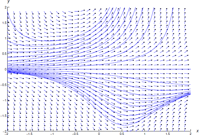
Solve the Bernoulli equation

\[\label{eq:2.4.3} y'-y=xy^2.\]

Solution

Dividing by \(y^2\) we get

\[y^{-2}y'-y^{-1}=x.\nonumber\]

If we now let \(u=y^{-1},\) we get \({du\over dx}=-y^{-2}{dy\over dx}\) and substituting into \ref{eq:2.4.3} we get

\[{-du\over dx}-u=x\nonumber\]

which is a linear equation. Putting it in standard linear form we get

\[{du\over dx}+u=-x\nonumber\]

and using the method of section 2.3 we get the solution

\[u=-{(x-1)+ce^{-x}} \nonumber\]

and substituting back in for u we get

\[y^{-1}=-{(x-1)+ce^{-x}} \nonumber\]

and solving for y we get our final solution

\[y=-{1\over x-1+ce^{-x}}. \nonumber\]

Figure 2.4.1 shows the direction field and some integral curves of Equation \ref{eq:2.4.3}.

Figure 2.4.1 : A direction field and integral curves for \(y'-y=xy^{2}\)

Homogeneous Equations

Definition 2.4.2

We say that a function \(f(x,y)\) is homogeneous of degree n if

\[f(tx,ty)=t^nf(x,y)\nonumber\]

Example \(\PageIndex{2}\)

Determine if \[f(x,y)=x^5+x^2y^3\nonumber\] is a homogeneous function and, if so, of what degree.

Solution

Substituting \(tx\) for \(x\) and \(ty\) for \(y\) we get \[f(tx,ty)=(tx)^5+(tx)^2(ty)^3=t^5(x^5+x^2y^3)=t^5f(x,y).\nonumber\] Therefore, \(f(x,y)\) is a homogeneous function of degree 5.

Example \(\PageIndex{3}\)

Determine if \[f(x,y)=x^2+xy^2\nonumber\] is a homogeneous function and, if so, of what degree.

Solution

Substituting \(tx\) for \(x\) and \(ty\) for \(y\) we get \[f(tx,ty)=(tx)^2+(tx)(ty)^2=t^2(x^2+txy^2)\ne t^nf(x,y).\nonumber\] for any number \(n\). Therefore, \(f(x,y)\) is not a homogeneous function.

Note: For this type of differential equation, as in section 2.2, it is convenient to write first order differential equations in the form

\[\label{eq:2.5.1} M(x,y)\,dx+N(x,y)\,dy=0.\]

Definition 2.4.3

We say that a differential equation of the form \(M(x,y)\,dx+N(x,y)\,dy=0\) is homogeneous if \(M(x,y)\) and \(N(x,y)\) are homogeneous functions of the same degree.

Example \(\PageIndex{4}\)

Determine if \[(x^2+xy)dx+y^2dy=0\nonumber\] is a homogeneous differential equation.

Solution

Substituting \(tx\) for \(x\) and \(ty\) for \(y\) in \(M(x,y)\) we get \[M(tx,ty)=(tx)^2+(tx)(ty)=t^2(x^2+xy)= t^2M(x,y)\nonumber\] and \(M(x,y)\) is a homogeneous function of degree 2.

Substituting \(tx\) for \(x\) and \(ty\) for \(y\) in \(N(x,y)\) we get \[N(tx,ty)=(ty)^2=t^2y^2= t^2N(x,y)\nonumber\] and \(N(x,y)\) is a homogeneous function of degree 2.

Since both \(M(x,y)\) and \(N(x,y)\) are homogeneous functions of degree 2, the differential equation is homogeneous.

Theorem \(\PageIndex{2}\)

The substitution \(y=ux\), where \(u\) is a function of \(x\), or \(x=vy\), where \(v\) is a function of \(y\) will make a homogeneous equation separable.

Proof

Note: we will only prove this for the substitution \(y=ux\) and leave the substitution \(x=vy\) to the reader.

Letting \[y=ux\nonumber\] and differentiating with respect to \(x\) we get

\[{dy\over dx}=u+x{du\over dx}\nonumber\] which can be rewritten as \[dy=udx+xdu.\nonumber\]

Substituting \(y\) and \(dy\) into \ref{eq:2.5.1} we get \[M(x,ux)dx+N(x,ux)[udx+xdu]=0.\nonumber\]

Using the fact that both \(M(x,y)\) and \(N(x,y)\) are homogeneous of the same degree we get

\[x^nM(1,u)dx+x^nN(1,u)[udx+xdu]=0.\nonumber\]

Expanding and rewriting this we eventually come to

\[x^n[M(1,u)+uN(1,u)]dx=-x^{n+1}N(1,u)du\nonumber\] which is clearly a separable differential equation:

\[{1\over x}dx={-N(1,u)\over M(1,u)+uN(1,u)}du.\nonumber\]

Example 2.4.5

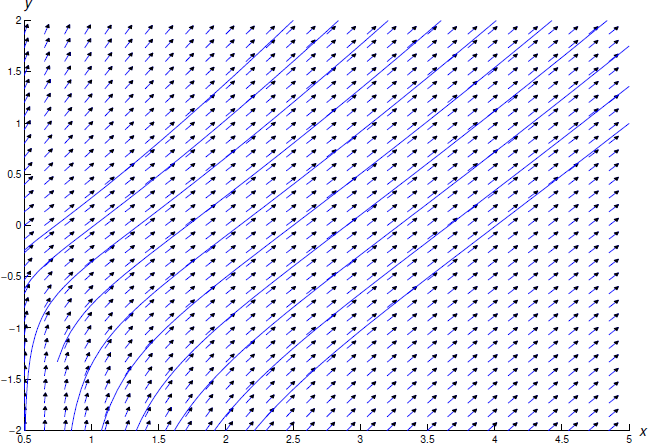
Solve

\[\label{eq:2.4.8} xdy=({y+xe^{-y/x}})dx.\]

First verify that \(M(x,y)\) and \(N(x,y)\) are homogeneous functions of the same degree.

Substituting \(y=ux\) into Equation \ref{eq:2.4.8} yields

\[x(udx+xdu)= ({ux+xe^{-ux/x}})dx.\nonumber\]

Simplifying and separating variables yields

\[e^udu={1\over x}dx. \nonumber\]

Integrating yields \(e^u=\ln |x|+c\). Therefore \(u=\ln(\ln|x|+c)\) and \(y=ux=x \ln (\ln |x|+c)\).

Figure 2.4.2 shows a direction field and integral curves for Equation \ref{eq:2.4.8}.

Figure 2.4.2 : A direction field and some integral curves for \(xdy=({y+xe^{-y/x}})dx\)

Equations of the form \({dy\over dx}=f(Ax+By+C)\)

Theorem \(\PageIndex{3}\)

The substitution \[u=Ax+By+C\nonumber\] will make equations of the form \[\label{eq:2.4.9} {dy\over dx}=f(Ax+By+C)\] separable.

Proof

Consider a differential equation of the form \ref{eq:2.4.9}.

Let \[u=Ax+By+C\nonumber\]

Taking the derivative with respect to x we get \[{du\over dx}=A+B{dy\over dx}.\nonumber\]

Substituting into \ref{eq:2.4.9} we get \[{1\over B}({du\over dx}-A)=f(u)\nonumber\]

which is clearly a separable differential equation: \[{du\over Bf(u)+A}=dx\nonumber\]

Example 2.4.6

Solve

\[\label{eq:2.4.10} y'=sec^2(y-x-3).\]

Solution

Letting \[u=y-x-3\nonumber\] and differentiating we get \[{du\over dx}={dy\over dx}-1\nonumber\]

Substituting into Equation \ref{eq:2.4.10} we get

\[{du\over dx}+1=sec^2u\nonumber\]

This is now a separable equation which can be solved using the method of section 2.1, resulting in a solution of

\[-\cot u-u=x+c\nonumber\]

and substituting in for u we get

\[-\cot (y-x-3)-(y-x-3)=x+c\nonumber\] and simplifying we get

\[\cot (y-x-3)=-y+c\nonumber\]