1.1: Systems of Linear Equations

Learning Objectives

• Relate the types of solution sets of a system of two (three) variables graphically to the intersections of lines in a plane (the intersection of planes in three space).
• Use elementary operations to find the solution to a linear system of equations algebraically.

Systems of Equations, Geometry

As you may remember, linear equations like \(2x+3y=6\) can be graphed as straight lines in the coordinate plane. We say that this equation is in two variables, in this case \(x\) and \(y\). Suppose you have two such equations, each of which can be graphed as a straight line, and consider the resulting graph of two lines. What would it mean if there exists a point of intersection between the two lines? This point, which lies on both graphs, gives \(x\) and \(y\) values for which both equations are true. In other words, this point gives the ordered pair (\(x,y\)) that satisfy both equations. If the point \(\left( x, y \right)\) is a point of intersection, we say that \(\left( x, y \right)\) is a solution to the two equations. In linear algebra, we often are concerned with finding the solution(s) to a system of equations, if such solutions exist. First, we consider graphical representations of solutions and later we will consider the algebraic methods for finding solutions.

When looking for the intersection of two lines in a graph, several situations may arise. The following picture (Figure \(\PageIndex{1}\)) demonstrates the possible situations when considering two equations (two lines in the graph) involving two variables.

Figure \(\PageIndex{1}\): The possibilities for a system with 2 equations and 2 variables: two crossing lines for one solution, two parallel lines for no solution, and two identical lines for infinitely many solutions. (CC BY-NC-SA 4.0; Kuttler via A First Course in LINEAR ALGEBRA)

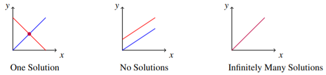
In the first diagram, there is a unique point of intersection, which means that there is only one (unique) solution to the two equations. In the second, there are no points of intersection and no solution. When no solution exists, this means that the two lines are parallel and they never intersect. The third situation which can occur, as demonstrated in diagram three, is that the two lines are really the same line. For example, \(x+y=1\) and \(2x+2y=2\) are equations which when graphed yield the same line. In this case there are infinitely many points which are solutions of these two equations, as every ordered pair which is on the graph of the line satisfies both equations. When considering linear systems of equations, there are always three types of solutions possible; exactly one (unique) solution, infinitely many solutions, or no solution.

Example \(\PageIndex{1}\): A Graphical Solution

Use a graph to find the solution to the following system of equations \[\begin{array}{c} x+y=3 \\ y-x=5 \end{array}\nonumber \]

Solution

Through graphing the above equations and identifying the point of intersection, we can find the solution(s). Remember that we must have either one solution, infinitely many, or no solutions at all. The following graph (Figure \(\PageIndex{2}\)) shows the two equations, as well as the intersection. Remember, the point of intersection represents the solution of the two equations, or the \(\left( x,y\right)\) which satisfy both equations. In this case, there is one point of intersection at \(\left( -1, 4 \right)\) which means we have one unique solution, \(x = -1, y = 4\).

Figure \(\PageIndex{2}\): The lines corresponding to the equations \(x+y=3\) and \(y-x=5\) intersect at \((-1,4)\). (CC BY-NC-SA 4.0; Kuttler via A First Course in LINEAR ALGEBRA)

In the above example, we investigated the intersection point of two equations in two variables, \(x\) and \(y\). Now we will consider the graphical solutions of three equations in two variables.

Consider a system of three equations in two variables. Again, these equations can be graphed as straight lines in the plane, so that the resulting graph contains three straight lines. Recall the three possible types of solutions; no solution, one solution, and infinitely many solutions. There are now more complex ways of achieving these situations, due to the presence of the third line. For example, you can imagine the case of three intersecting lines having no common point of intersection. Perhaps you can also imagine three intersecting lines which do intersect at a single point. These two situations are illustrated below (Figure \(\PageIndex{3}\)).

Figure \(\PageIndex{3}\): The first diagram shows a linear system corresponding to three pairwise non-parallel lines with no common point of intersection has no solution. The second diagram shows linear system corresponding to three pairwise non-parallel lines with one common point of intersection has one solution. (CC BY-NC-SA 4.0; Kuttler via A First Course in LINEAR ALGEBRA)

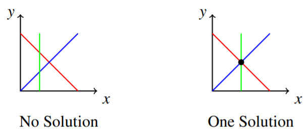
Consider the first picture above. While all three lines intersect with one another, there is no common point of intersection where all three lines meet at one point. Hence, there is no solution to the three equations. Remember, a solution is a point \(\left( x, y \right)\) which satisfies all three equations. In the case of the second picture, the lines intersect at a common point. This means that there is one solution to the three equations whose graphs are the given lines. You should take a moment now to draw the graph of a system which results in three parallel lines. Next, try the graph of three identical lines. Which type of solution is represented in each of these graphs?

We have now considered the graphical solutions of systems of two equations in two variables, as well as three equations in two variables. However, there is no reason to limit our investigation to equations in two variables. We will now consider equations in three variables.

You may recall that equations in three variables, such as \(2x+4y-5z=8\), form a plane. Above, we were looking for intersections of lines in order to identify any possible solutions. When graphically solving systems of equations in three variables, we look for intersections of planes. These points of intersection give the \(\left( x, y, z \right)\) that satisfy all the equations in the system. What types of solutions are possible when working with three variables? Consider the following picture involving two planes, which are given by two equations in three variables (Figure \(\PageIndex{4}\)).

Figure \(\PageIndex{4}\): Two planes intersecting in a line. (CC BY-NC-SA 4.0; Kuttler via A First Course in LINEAR ALGEBRA)

Notice how these two planes intersect in a line. This means that the points \(\left( x,y,z\right)\) on this line satisfy both equations in the system. Since the line contains infinitely many points, this system has infinitely many solutions.

It could also happen that the two planes fail to intersect. However, is it possible to have two planes intersect at a single point? Take a moment to attempt drawing this situation, and convince yourself that it is not possible! This means that when we have only two equations in three variables, there is no way to have a unique solution! Hence, the types of solutions possible for two equations in three variables are no solution or infinitely many solutions.

Now imagine adding a third plane. In other words, consider three equations in three variables. What types of solutions are now possible? Consider the following diagram (Figure \(\PageIndex{5}\)).

Figure \(\PageIndex{5}\): A third plane added to the system of two planes from Figure \(\PageIndex{4}\) that intersected in a line. The third plane is parallel to one of the original planes, which results in no common points of intersection. (CC BY-NC-SA 4.0; Kuttler via A First Course in LINEAR ALGEBRA)

In this diagram, there is no point which lies in all three planes. There is no intersection between all planes so there is no solution. The picture illustrates the situation in which the line of intersection of the new plane with one of the original planes forms a line parallel to the line of intersection of the first two planes. However, in three dimensions, it is possible for two lines to fail to intersect even though they are not parallel. Such lines are called skew lines.

Recall that when working with two equations in three variables, it was not possible to have a unique solution. Is it possible when considering three equations in three variables? In fact, it is possible, and we demonstrate this situation in the following picture (Figure \(\PageIndex{6}\)).

Figure \(\PageIndex{6}\): A third plane added to the system of two planes from Figure \(\PageIndex{4}\) that intersected in a line. The third plane is perpendicular to one of the original planes, which results in one point of intersection. (CC BY-NC-SA 4.0; Kuttler via A First Course in LINEAR ALGEBRA)

In this case, the three planes have a single point of intersection. Can you think of other types of solutions possible? Another is that the three planes could intersect in a line, resulting in infinitely many solutions, as in the following diagram (Figure \(\PageIndex{7}\)).

Figure \(\PageIndex{7}\): A third plane added to the system of two planes from Figure \(\PageIndex{4}\) that intersected in a line. The third plane passes through the line of intersection, which results all three planes intersecting in that line. (CC BY-NC-SA 4.0; Kuttler via A First Course in LINEAR ALGEBRA)

We have now seen how three equations in three variables can have no solution, a unique solution, or intersect in a line resulting in infinitely many solutions. It is also possible that the three equations graph the same plane, which also leads to infinitely many solutions.

You can see that when working with equations in three variables, there are many more ways to achieve the different types of solutions than when working with two variables. It may prove enlightening to spend time imagining (and drawing) many possible scenarios, and you should take some time to try a few.

You should also take some time to imagine (and draw) graphs of systems in more than three variables. Equations like \(x+y-2z+4w=8\) with more than three variables are often called hyper-planes. You may soon realize that it is tricky to draw the graphs of hyper-planes! Through the tools of linear algebra, we can algebraically examine these types of systems which are difficult to graph. In the following section, we will consider these algebraic tools.

Algebraic Procedures

We have taken an in depth look at graphical representations of systems of equations, as well as how to find possible solutions graphically. Our attention now turns to working with systems algebraically.

Definition \(\PageIndex{1}\): System of Linear Equations

A system of linear equations is a list of equations, \[\begin{array}{c} a_{11}x_{1}+a_{12}x_{2}+\cdots +a_{1n}x_{n}=b_{1} \\ a_{21}x_{1}+a_{22}x_{2}+\cdots +a_{2n}x_{n}=b_{2} \\ \vdots \\ a_{m1}x_{1}+a_{m2}x_{2}+\cdots +a_{mn}x_{n}=b_{m} \end{array}\nonumber\] where \(a_{ij}\) and \(b_{j}\) are real numbers. The above is a system of \(m\) equations in the \(n\) variables, \(x_{1},x_{2}\cdots ,x_{n}\). Written more simply in terms of summation notation, the above can be written in the form \[\sum_{j=1}^{n}a_{ij}x_{j}=b_{i}, \text{ }i=1,2,3,\cdots ,m\nonumber\]

The relative size of \(m\) and \(n\) is not important here. Notice that we have allowed \(a_{ij}\) and \(b_{j}\) to be any real number. We can also call these numbers scalars . We will use this term throughout the text, so keep in mind that the term scalar just means that we are working with real numbers.

Now, suppose we have a system where \(b_{i} = 0\) for all \(i\). In other words every equation equals \(0\). This is a special type of system.

Definition \(\PageIndex{2}\): Homogeneous System of Equations

A system of equations is called homogeneous if each equation in the system is equal to \(0\). A homogeneous system has the form \[\begin{array}{c} a_{11}x_{1}+a_{12}x_{2}+\cdots +a_{1n}x_{n}= 0 \\ a_{21}x_{1}+a_{22}x_{2}+\cdots +a_{2n}x_{n}= 0 \\ \vdots \\ a_{m1}x_{1}+a_{m2}x_{2}+\cdots +a_{mn}x_{n}= 0 \end{array}\nonumber \] where \(a_{ij}\) are scalars and \(x_{i}\) are variables.

Recall from the previous section that our goal when working with systems of linear equations was to find the point of intersection of the equations when graphed. In other words, we looked for the solutions to the system. We now wish to find these solutions algebraically. We want to find values for \(x_{1},\cdots ,x_{n}\) which solve all of the equations. If such a set of values exists, we call \(\left( x_{1},\cdots ,x_{n}\right)\) the solution set.

Recall the above discussions about the types of solutions possible. We will see that systems of linear equations will have one unique solution, infinitely many solutions, or no solution. Consider the following definition.

Definition \(\PageIndex{3}\): Consistent and Inconsistent Systems

A system of linear equations is called consistent if there exists at least one solution. It is called inconsistent if there is no solution.

If you think of each equation as a condition which must be satisfied by the variables, consistent would mean there is some choice of variables which can satisfy all the conditions. Inconsistent would mean there is no choice of the variables which can satisfy all of the conditions.

The following sections provide methods for determining if a system is consistent or inconsistent, and finding solutions if they exist.

Elementary Operations

We begin with an example. Recall from Example 1.1.1 that the solution to the given system was \(\left(x, y \right) = \left( -1, 4 \right)\).

Example \(\PageIndex{2}\): Verifying an Ordered Pair is a Solution

Algebraically verify that \(\left(x, y \right) = \left( -1, 4 \right)\) is a solution to the following system of equations.

\[\begin{array}{c} x+y=3 \\ y-x=5 \end{array}\nonumber \]

Solution

By graphing these two equations and identifying the point of intersection, we previously found that \(\left(x, y \right) = \left( -1, 4 \right)\) is the unique solution.

We can verify algebraically by substituting these values into the original equations, and ensuring that the equations hold. First, we substitute the values into the first equation and check that it equals \(3\). \[x + y = (-1)+(4) = 3\nonumber \] This equals \(3\) as needed, so we see that \(\left( -1,4 \right)\) is a solution to the first equation. Substituting the values into the second equation yields \[y -x = (4) - (-1) = 4 + 1 = 5\nonumber \] which is true. For \(\left( x,y\right) =\left( -1,4\right)\) each equation is true and therefore, this is a solution to the system.

Now, the interesting question is this: If you were not given these numbers to verify, how could you algebraically determine the solution? Linear algebra gives us the tools needed to answer this question. The following basic operations are important tools that we will utilize.

Definition \(\PageIndex{4}\): Elementary Operations

Elementary operations are those operations consisting of the following.

1. Interchange the order in which the equations are listed.
2. Multiply any equation by a nonzero number.
3. Replace any equation with itself added to a multiple of another equation.

It is important to note that none of these operations will change the set of solutions of the system of equations. In fact, elementary operations are the key tool we use in linear algebra to find solutions to systems of equations.

Consider the following example.

Example \(\PageIndex{3}\): Effects of an Elementary Operation

Show that the system \[\begin{array}{c} x+y=7 \\ 2x-y=8 \end{array}\nonumber \] has the same solution as the system \[\begin{array}{c} x+y=7 \\ -3y=-6 \end{array}\nonumber \]

Solution

Notice that the second system has been obtained by taking the second equation of the first system and adding -2 times the first equation, as follows: \[2x-y + (-2)(x+y) = 8 + (-2)(7)\nonumber \] By simplifying, we obtain \[-3y=-6\nonumber \] which is the second equation in the second system. Now, from here we can solve for \(y\) and see that \(y=2\). Next, we substitute this value into the first equation as follows \[x+y=x+2=7\nonumber \] Hence \(x=5\) and so \(\left( x,y\right) = \left(5,2 \right)\) is a solution to the second system. We want to check if \(\left(5,2 \right)\) is also a solution to the first system. We check this by substituting \(\left(x, y \right) = \left(5,2 \right)\) into the system and ensuring the equations are true. \[\begin{array}{c} x+y = \left(5 \right)+ \left( 2 \right) = 7 \\ 2x-y= 2 \left(5 \right) - \left( 2 \right) = 8 \end{array}\nonumber \] Hence, \(\left(5,2 \right)\) is also a solution to the first system.

This example illustrates how an elementary operation applied to a system of two equations in two variables does not affect the solution set. However, a linear system may involve many equations and many variables and there is no reason to limit our study to small systems. For any size of system in any number of variables, the solution set is still the collection of solutions to the equations. In every case, the above operations of Definition \(\PageIndex{4}\) do not change the set of solutions to the system of linear equations.

In the following theorem, we use the notation \(E_i\) to represent an equation, while \(b_i\) denotes a constant.

Theorem \(\PageIndex{1}\): Elementary Operations and Solutions

Suppose you have a system of two linear equations \[\begin{array}{c} E_{1}=b_{1}\\ E_{2}=b_{2} \end{array} \label{system}\] Then the following systems have the same solution set:

1. \[\begin{array}{c} E_{2}=b_{2}\\ E_{1}=b_{1} \end{array} \label{thm1.9.1}\]
2. \[\begin{array}{c} E_{1}=b_{1} \\ kE_{2}=kb_{2}\\ \end{array} \label{thm1.9.2}\] for any scalar \(k\), provided \(k\neq0\).
3. \[\begin{array}{c} E_{1}=b_{1} \\ E_{2}+kE_{1}=b_{2}+kb_{1} \end{array} \label{thm1.9.3}\] for any scalar \(k\) (including \(k=0\)).

Before we proceed with the proof of Theorem \(\PageIndex{1}\), let us consider this theorem in context of Example \(\PageIndex{3}\). Then, \[\begin{array}{cc} E_{1} = x+y, & b_{1} = 7 \\ E_{2} = 2x-y, & b_{2} = 8 \end{array}\nonumber \] Recall the elementary operations that we used to modify the system in the solution to the example. First, we added \(\left( -2 \right)\) times the first equation to the second equation. In terms of Theorem \(\PageIndex{1}\), this action is given by \[E_{2} + \left( -2 \right) E_{1} = b_{2} + \left( -2 \right)b_{1}\nonumber \] or \[2x-y + \left( -2 \right) \left(x+y \right) = 8 + \left( -2 \right) 7\nonumber \] This gave us the second system in Example \(\PageIndex{3}\), given by \[\begin{array}{c} E_{1} = b_{1} \\ E_{2} + \left( -2 \right) E_{1} = b_{2} + \left( -2 \right) b_{1} \end{array}\nonumber \]

From this point, we were able to find the solution to the system. Theorem \(\PageIndex{1}\) tells us that the solution we found is in fact a solution to the original system.

We will now prove Theorem \(\PageIndex{1}\).

Theorem \(\PageIndex{1}\)

Proof

1. The proof that the systems \(\eqref{system}\) and \(\eqref{thm1.9.1}\) have the same solution set is as follows. Suppose that \(\left( x_{1},\cdots ,x_{n}\right)\) is a solution to \(E_{1}=b_{1},E_{2}=b_{2}\). We want to show that this is a solution to the system in \(\eqref{thm1.9.1}\) above. This is clear, because the system in \(\eqref{thm1.9.1}\) is the original system, but listed in a different order. Changing the order does not effect the solution set, so \(\left( x_{1},\cdots ,x_{n}\right)\) is a solution to \(\eqref{thm1.9.1}\).
2. Next we want to prove that the systems \(\eqref{system}\) and \(\eqref{thm1.9.2}\) have the same solution set. That is \(E_{1}=b_{1},E_{2}=b_{2}\) has the same solution set as the system \(E_{1}=b_{1},kE_{2}=kb_{2}\) provided \(k\neq 0\). Let \(\left( x_{1},\cdots ,x_{n}\right)\) be a solution of \(E_{1}=b_{1},E_{2}=b_{2},\). We want to show that it is a solution to \(E_{1}=b_{1},kE_{2}=kb_{2}\). Notice that the only difference between these two systems is that the second involves multiplying the equation, \(E_{2}=b_{2}\) by the scalar \(k\). Recall that when you multiply both sides of an equation by the same number, the sides are still equal to each other. Hence if \(\left( x_{1},\cdots ,x_{n}\right)\) is a solution to \(E_{2}=b_{2}\), then it will also be a solution to \(kE_{2}=kb_{2}\). Hence, \(\left( x_{1},\cdots ,x_{n}\right)\) is also a solution to \(\eqref{thm1.9.2}\). Similarly, let \(\left( x_{1},\cdots ,x_{n}\right)\) be a solution of \(E_{1}=b_{1},kE_{2}=kb_{2}\). Then we can multiply the equation \(kE_{2}=kb_{2}\) by the scalar \(1/k\), which is possible only because we have required that \(k\neq 0\). Just as above, this action preserves equality and we obtain the equation \(E_{2} = b_{2}\). Hence \(\left( x_{1},\cdots ,x_{n}\right)\) is also a solution to \(E_{1}=b_{1},E_{2}=b_{2}.\)
3. Finally, we will prove that the systems \(\eqref{system}\) and \(\eqref{thm1.9.3}\) have the same solution set. We will show that any solution of \(E_{1}=b_{1},E_{2}=b_{2}\) is also a solution of \(\eqref{thm1.9.3}\). Then, we will show that any solution of \(\eqref{thm1.9.3}\) is also a solution of \(E_{1}=b_{1},E_{2}=b_{2}\). Let \(\left( x_{1},\cdots ,x_{n}\right)\) be a solution to \(E_{1}=b_{1},E_{2}=b_{2}\). Then in particular it solves \(E_{1} = b_{1}\). Hence, it solves the first equation in \(\eqref{thm1.9.3}\). Similarly, it also solves \(E_{2} = b_{2}\). By our proof of \(\eqref{thm1.9.2}\), it also solves \(kE_{1}=kb_{1}\). Notice that if we add \(E_{2}\) and \(kE_{1}\), this is equal to \(b_{2} + kb_{1}\). Therefore, if \(\left( x_{1},\cdots ,x_{n}\right)\) solves \(E_{1}=b_{1},E_{2}=b_{2}\) it must also solve \(E_{2}+kE_{1}=b_{2}+kb_{1}\). Now suppose \(\left( x_{1},\cdots ,x_{n}\right)\) solves the system \(E_{1}=b_{1}, E_{2}+kE_{1}=b_{2}+kb_{1}\). Then in particular it is a solution of \(E_{1} = b_{1}\). Again by our proof of \(\eqref{thm1.9.2}\), it is also a solution to \(kE_{1}=kb_{1}\). Now if we subtract these equal quantities from both sides of \(E_{2}+kE_{1}=b_{2}+kb_{1}\) we obtain \(E_{2}=b_{2}\), which shows that the solution also satisfies \(E_{1}=b_{1},E_{2}=b_{2}.\

Stated simply, the above theorem shows that the elementary operations do not change the solution set of a system of equations.

We will now look at an example of a system of three equations and three variables. Similarly to the previous examples, the goal is to find values for \(x,y,z\) such that each of the given equations are satisfied when these values are substituted in.

Example \(\PageIndex{4}\): Solving a System of Equations with Elementary Operations

Find the solutions to the system,

\[\begin{array}{c} x+3y+6z=25 \\ 2x+7y+14z=58 \\ 2y+5z=19 \end{array} \label{solvingasystem1}\]

Solution

We can relate this system to Theorem \(\PageIndex{1}\) above. In this case, we have \[\begin{array}{c c} E_{1} = x + 3y + 6z, & b_{1} = 25\\ E_{2} = 2x+7y+14z, & b_{2} = 58 \\ E_{3} = 2y+5z, & b_{3} = 19 \end{array}\nonumber \] Theorem \(\PageIndex{1}\) claims that if we do elementary operations on this system, we will not change the solution set. Therefore, we can solve this system using the elementary operations given in Definition \(\PageIndex{4}\). First, replace the second equation by \(\left( -2\right)\) times the first equation added to the second. This yields the system \[\begin{array}{c} x+3y+6z=25 \\ y+2z=8 \\ 2y+5z=19 \end{array} \label{solvingasystem2}\] Now, replace the third equation with \(\left( -2\right)\) times the second added to the third. This yields the system \[\begin{array}{c} x+3y+6z=25 \\ y+2z=8 \\ z=3 \end{array} \label{solvingasystem3}\] At this point, we can easily find the solution. Simply take \(z=3\) and substitute this back into the previous equation to solve for \(y\), and similarly to solve for \(x\). \[\begin{array}{c} x + 3y + 6 \left(3 \right) = x + 3y + 18 = 25\\ y + 2 \left(3 \right) = y + 6 = 8 \\ z = 3 \end{array}\nonumber \] The second equation is now \[y+6=8\nonumber \] You can see from this equation that \(y = 2\). Therefore, we can substitute this value into the first equation as follows: \[x + 3 \left(2 \right) + 18 = 25\nonumber \] By simplifying this equation, we find that \(x=1\). Hence, the solution to this system is \(\left( x,y,z \right) = \left( 1,2,3 \right)\). This process is called back substitution.

Alternatively, in \(\eqref{solvingasystem3}\) you could have continued as follows. Add \(\left( -2\right)\) times the third equation to the second and then add \(\left( -6\right)\) times the second to the first. This yields \[ \begin{array}{c} x+3y=7 \\ y=2 \\ z=3 \end{array}\nonumber \] Now add \(\left( -3\right)\) times the second to the first. This yields \[ \begin{array}{c} x=1 \\ y=2 \\ z=3 \end{array}\nonumber \] a system which has the same solution set as the original system. This avoided back substitution and led to the same solution set. It is your decision which you prefer to use, as both methods lead to the correct solution, \(\left( x,y,z \right) = \left(1,2,3\right)\).