6.A: Answers

Section 6.1

1. \(y = e^{-3x}+2 \Rightarrow y' = -3e^{-3x}\) so \(y'+3y = \left(-3e^{-3x}\right)+3\left(e^{-3x}+2\right) = -3e^{-3x}+3e^{-3x}+6 = 6\)
3. \(y=x^2+2x \Rightarrow y' = 2x+2 \Rightarrow y' = 2\) so \(y''-y'+y=2-\left(2x+2\right)+\left(x^2+2x\right) = 2-2x-2+x^2+2x = x^2\)
5. \(y=7x^3-x^2 \Rightarrow y' = 21x^2-2x\) so \(xy'-3y=x\left(21x^2-2x\right)-3\left(7x^3-x^2\right) = 21x^3-2x^2-21x^3+3x^2=x^2\)
7. \(y = \frac12 e^{x}+2e^{-x} \Rightarrow y' = \frac12 e^x - 2 e^{-x}\) so \(y'+y = \left(\frac12 e^x - 2 e^{-x}\right)+\left(\frac12 e^{x}+2e^{-x}\right) = e^x\)
9. \(\displaystyle y = \left(7-x^2\right)^{\frac12} \Rightarrow y' = \frac12\left(7-x^2\right)^{-\frac12}\left(-2x\right) = \frac{-x}{\sqrt{7-x^2}} = -\frac{x}{y}\)
11. \(y = 2x^3-3x+3 \Rightarrow y(1) = 2\cdot 1^3 - 3\cdot 1 + 3 = 2\) (OK) and \(y' = 6x^2-3\) (OK)
13. \(y = \sin(2x)+1 \Rightarrow y(0)=\sin(0)+1=1\) (OK) and \(y'=2\cos(2x)\) (OK)
15. \(y = 7e^{5x} \Rightarrow y(0) = 7e^{5\cdot 0} = 7\) (OK) and \(y' = 7e^{5x}\cdot 5 - 5y\) (OK)
17. \(\displaystyle y = -\frac{4}{x} \Rightarrow y(1) = -\frac{4}{1} = -4\) (OK) and \(\displaystyle y' = \frac{4}{x^2}\) so \(\displaystyle x\cdot y' = x\left(\frac{4}{x^2}\right) = \frac{4}{x} = -y\)
19. \(y = 5\ln(x)-2 \Rightarrow y(e) = 5\ln(e)-2 = 5-2=3\) (OK) and \(\displaystyle y' = 5\cdot\frac{1}{x}\) (OK)
21. \(7 = y(3) = 3^2+C = 9 +C \Rightarrow C = -2\)
23. \(5 = y(0) = Ce^{3\cdot 0} = C\cdot 1 \Rightarrow C = 5\)
25. \(4 = y(0) =2\sin(3\cdot 0) + C = 0 + C \Rightarrow C = 4\)
27. \(2 = y(e) = \ln(e) + C = 1 + C \Rightarrow C = 1\)
29. \(\displaystyle 10 = y(2) =-\frac{C}{2} \Rightarrow C = -20\)
31. \(\displaystyle y = \int\left[4x^2-x\right]\, dx = \frac43 x^3 - \frac12 x^2 + C\) so \(7 = y(1) = \frac43 - \frac12 + C \Rightarrow C = \frac{37}{6}\) and \(y = \frac43 x^3 - \frac12 x^2 + \frac{37}{6}\)
33. \(\displaystyle y = \int \frac{3}{x}\, dx = 3\ln\left(\left|x\right|\right) + C\) so \(2 = y(1) = 3\ln(1) + C = 0 + C\) so \(C +2\) and \(y = 3\ln\left(\left|x\right|\right) + 2\)
35. \(\displaystyle y = \int 6e^{2x} \, dx = 3e^{2x} + C\) so \(1 = y(0) = 3e^{2\cdot 0} + C = 3+C \Rightarrow C = -2\) and \(y = 3e^{2x} - 2\)
37. \(\displaystyle y = \int x\cdot\sin\left(x^2\right)\, dx = -\frac12 \cos\left(x^2\right) + C\) so \(3 = y(0) = -\frac12 \cos(0)+C = -\frac12 + C \Rightarrow C = \frac72\) and \(\displaystyle y = -\frac12 \cos\left(x^2\right) + \frac72\)
39. \(\displaystyle y' = \frac{1}{x}\left(6x^3-10x^2\right) = 6x^2-10x \Rightarrow y = \int\left[6x^2-10x\right]\, dx = 2x^3-5x^2+C\) so \(5 = y(2) = 2\cdot 2^3 - 5\cdot 2^2 + C = 16-20+C = -4 + C \Rightarrow C = 9\) and \(y = 2x^3-5x^2+9\)
41. We know that \(f'(x)+5\cdot f(x) =0\) and \(g'(x)+5\cdot g(x) =0\), so: \(y = 3f(x) \Rightarrow y' = 3f'(x) \Rightarrow y'+5y=3f'(x) + 5\cdot 3f(x) = 3\left[f'(x) + 5 \cdot f(x)\right] = 3\cdot 0 = 0\)
    \(y = 7g(x) \Rightarrow y' = 7g'(x) \Rightarrow y'+5y=7g'(x) + 5\cdot 7g(x) = 7\left[g'(x) + 5 \cdot g(x)\right] = 3\cdot 0\)
    \(y = f(x)+g(x) \Rightarrow y' = f'(x)+g'(x) \Rightarrow y'+5\cdot y = \left[f'(x)+g'(x)\right] + 5\cdot\left[f(x)+g(x)\right] \Rightarrow y = f'(x) + g'(x) + 5f(x) + 5g(x) = \left[f'(x) + 5f(x)\right] + \left[g'(x) + 5g(x)\right] = 0+0 = 0\)
    \(y = A\cdot f(x) + B\cdot g(x) \Rightarrow y' = A\cdot f'(x)+B \cdot g'(x) \Rightarrow y'+5\cdot y = \left[A\cdot f'(x)+B\cdot g'(x)\right] + 5\cdot\left[A\cdot f(x)+B\cdot g(x)\right] \Rightarrow y = Af'(x) + Bg'(x) + 5Af(x) + 5Bg(x) = A\left[f'(x) + 5f(x)\right] + B\left[g'(x) + 5g(x)\right] = A\cdot 0+B\cdot 0 = 0\)
43. \(y = \sin(x) + x \Rightarrow y' = \cos(x) + 1 \Rightarrow y'' = -\sin(x) \Rightarrow y''+y = \left[-\sin(x)\right]+\left[\sin(x) + x\right] = x\)
    \(y = \cos(x) + x \Rightarrow y' = -\sin(x) + 1 \Rightarrow y'' = -\cos(x) \Rightarrow y''+y = \left[-\cos(x)\right]+\left[\cos(x) + x\right] = x\) (OK)
    \(y = 3\left[\sin(x) + x\right] \Rightarrow y' = 3\cos(x) + 3 \Rightarrow y'' = -3\sin(x) \Rightarrow y''+y = -3\sin(x) +3\left[\sin(x) + x\right] = 3x\) (NO)
    Similarly, \(y = \left[\sin(x) + x\right]+\left[\cos(x) + x\right] \Rightarrow y''+y =2x\) (NO)
45. \(y = \frac{A}{B}-C\cdot e^{-Bt} \Rightarrow \frac{dy}{dt} = 0 - C\left[-Be^{-Bt}\right] = BCe^{-Bt} \Rightarrow A-By = A - B \left[ \frac{A}{B}-C\cdot e^{-Bt}\right] = A - A +BCe^{-Bt} = BCe^{-Bt} = \frac{dy}{dt}\) (OK)
47. \(I = \frac{E}{R}\left[1-\cdot e^{-\frac{Rt}{L}}\right] \Rightarrow \frac{dI}{dt} = \frac{E}{R}\left[0 - \left(-\frac{R}{L}\right)e^{-\frac{Rt}{L}}\right] = \frac{E}{R}e^{-\frac{Rt}{L}} \Rightarrow L\cdot\frac{dI}{dt} + R\cdot I = l\left[\frac{E}{R}e^{-\frac{Rt}{L}}\right] + r\cdot \frac{E}{R}\left[1-\cdot e^{-\frac{Rt}{L}}\right] = E\cdot e^{-\frac{Rt}{L}}+E\left[1-e^{-\frac{Rt}{L}}\right] = E\) (OK)

Section 6.2

1. 
3. 
5. 
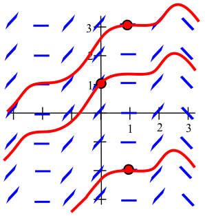
6. All solutions appear to approach the horizontal line \(y=1\): for any solution \(y(x)\), \(\displaystyle \lim_{x \to \infty} \, y(x) = 1\).
9. 
11. 
13. 
15. 1. \(y = x^2-3x+C\)
    2. \(4 = y(1) = 1^2-3\cdot 1 + C \Rightarrow 4 = C- 2 \Rightarrow C = 6\) so \(y = x^2-3x+6\)
    3. \((-\infty, \infty)\)
17. 1. \(\Rightarrow y = e^x + \sin(x) + C\)
    2. \(7 = y(0) = 1+0 + C \Rightarrow C = 6\) so \(y = e^x+\sin(x)+6\)
    3. \((-\infty, \infty)\)
19. 1. \(\displaystyle y' = \frac{6}{2x+1} + \sqrt{x} \Rightarrow y = 3\ln\left(\left|2x+1\right|\right) + \frac23 x^{\frac32} + C\)
    2. \(4 = y(1) = 3\ln(3) + \frac23 + C \Rightarrow C = \frac{10}{3}-3\ln(3)\) so \(3\ln\left(\left|2x+1\right|\right) + \frac23 x^{\frac32} + \frac{10}{3}-3\ln(3)\)
    3. \((0, \infty)\)
21. 
23. 

Section 6.3

1. 
3. If \(y \neq 0\), divide both sides by \(y\) to separate:\[\frac{1}{y}\cdot \frac{dy}{dx} = 2x \Rightarrow \frac{1}{y}\, dy = 2x \, dx\nonumber\]and then integrate both sides:\[\int \frac{1}{y}\, dy = \int 2x \, dx \Rightarrow \ln\left(\left|y\right|\right) = x^2 + C\nonumber\]then exponentiate both sides to solve for \(y\):\[e^{\ln\left(\left|y\right|\right)} = e^{x^2 + C} \Rightarrow \left|y\right| = e^C \cdot e^{x^2} \Rightarrow y = \pm e^C \cdot e^{x^2}\nonumber\]so \(\displaystyle y = A e^{x^2}\) is a solution for any \(A \neq 0\). But the constant function \(y(x) = 0\) is also a solution to \(y' = 2xy\) so the general solution is \(y = A e^{x^2}\) for any constant \(A\).
5. Divide both sides of the ODE by \(1+x^2\) to separate, then integrate:\[\frac{dy}{dx} = \frac{3}{1+x^2} \Rightarrow y = 3\arctan(x) + C\nonumber\]
7. Divide both sides by \(e^{y} \cdot \cos(x)\) to separate:\[\frac{1}{e^y} \cdot \frac{dy}{dx} = \frac{1}{\cos(x)} \Rightarrow e^{-y} \, dy = \sec(x) \, dx\nonumber\]and use Appendix I to assist with the integration: \begin{align*} \int e^{-y} \, dy &= \int \sec(x) \, dx\\ &\Rightarrow -e^{-y} = \ln\left(\left|\sec(x)+\tan(x)\right|\right) + C\end{align*} then solve for \(y\): \begin{align*}e^{-y} &= K-\ln\left(\left|\sec(x)+\tan(x)\right|\right) \Rightarrow \\ -y &= \ln\left( K-\ln\left(\left|\sec(x)+\tan(x)\right|\right)\right)\end{align*} so the general solution is:\[y = -\ln\left( K-\ln\left(\left|\sec(x)+\tan(x)\right|\right)\right)\nonumber\]
9. Note that \(y = 0\) is a solution to \(y' = 4y\). If \(y \neq 0\), divide both sides of the ODE by \(y\) to separate:\[\frac{1}{y} \cdot \frac{dy}{dx} = 4 \Rightarrow \frac{1}{y}\, dy = 4\, dx\nonumber\]then integrate both sides:\[\int \frac{1}{y}\, dy = \int 4\, dx \Rightarrow \ln\left(\left|y\right|\right) = 4x + C\nonumber\]and solve for \(y\):\[e^{\ln\left(\left|y\right|\right)} = e^{4x + C} \Rightarrow \left|y\right| = e^C \cdot e^{4x} \Rightarrow y = \pm e^C \cdot e^{4x}\nonumber\]so \(y = A e^{4x}\) is a solution for any constant \(A \neq 0\) but \(y(x) = 0\) is also a solution, so the general solution is \(y(x) = Ae^{4x}\) for any constant \(A\).
11. From Problem 3, we know that \(\displaystyle y = A e^{x^2}\), so using each initial condition: \begin{align*} 3 &= y(0) = A\cdot e^{0^2} = A \Rightarrow A = 3 \Rightarrow y = 3e^{x^2}\\ 5 &= y(0) = A\cdot e^{0^2} = A \Rightarrow A = 5 \Rightarrow y = 5e^{x^2}\\ 2 &= y(1) = A\cdot e \Rightarrow A = 2e^{-1} \Rightarrow y = 2e^{x^2-1} \end{align*}
13. Mimic the solution to Problem 9 to arrive at the general solution: \(\displaystyle y = A e^{3x}\). Then use each initial condition: \begin{align*} 4 &= y(0) = A\cdot e^{3\cdot 0} = A \Rightarrow A = 4 \Rightarrow y = 4e^{3x}\\ 7 &= y(0) = A\cdot e^{3\cdot 0} = A \Rightarrow A = 7 \Rightarrow y = 7e^{3x}\\ 3 &= y(1) = A\cdot e^{3\cdot 1} = Ae^3 \Rightarrow A = 3e^{-3} \Rightarrow y = 3e^{3x-3} \end{align*}
15. From Problem 10, we know \(\displaystyle y = 2+Ae^{-5x}\), so using each initial condition: \begin{align*} 5 &= y(0) = 2+A \cdot 1 \Rightarrow A = 3 \Rightarrow y = 2+3e^{-5x}\\ -3 &= y(0) = 2+A\cdot 1 \Rightarrow A = -5 \Rightarrow y = 2-5e^{-5x} \end{align*}
17. From Problem 5, we know \(\displaystyle y = 3\arctan(x)+C\), so using each initial condition: \begin{align*} 4 &= y(1) = 3\cdot \frac{\pi}{4} + C \Rightarrow y = 3\arctan(x) + 4 - \frac{3\pi}{4}\\ 2 &= y(0) = 3\cdot 0 + C \Rightarrow y = 3\arctan(x)+2 \end{align*}
19. No. Putting \(x = 0\) and \(y = 2\) into the ODE:\[0\cdot y'(0) = 2+3 \Rightarrow 0 = 5\nonumber\]which is a contradiction.

Section 6.4

1. The population is 10,000 around 1966 and is 20,000 around 1978, so \(1978-1966 = 12\) years. The population grows from 15,000 around 1974 to 30,000 around 1985, so \(1985-1974 = 11\) years. The doubling time is approximately 12 years.
3. 1. If \(P(t)\) represents the population (in thousands) \(t\) years after 1990, then \(\displaystyle P(t) = 48e^{kt}\) for some constant \(k\). We also know that:\[64 = 48 e^{20k} \ \Rightarrow \ \frac43 = e^{20k} \ \Rightarrow \ k = \frac{1}{20}\ln\left(\frac43\right)\nonumber\]so that \(\displaystyle P(t) = 48\left(\frac43\right)^{\frac{t}{20}} \approx 48e^{0.01438t}\).
   2. \(\displaystyle P(30)= 48\left(\frac43\right)^{\frac{30}{20}} \approx 73.901\), so if the model holds, in 2020 the community's population will be approximately 74,000.
   3. Solving \(P(t)=100\) for \(t\): \begin{align*} &100 = 48\left(\frac43\right)^{\frac{t}{20}} \ \Rightarrow \ \frac{100}{48} = \left(\frac43\right)^{\frac{t}{20}} \\ &\Rightarrow \ \ln\left(\frac{25}{12}\right) = \frac{t}{20}\ln\left(\frac43\right) \ \Rightarrow t = \frac{20\ln\left(\frac{25}{12}\right)}{\ln\left(\frac43\right)} \end{align*} so about 51 years later (in 2041).
   4. \(\displaystyle \frac{\ln(2)}{k} = \frac{20\ln(2)}{\ln\left(\frac43\right)} \approx 48.19\) years
5. If \(A(t)\) is the value of the investment \(t\) years later:\[A(t) = 5000(1.15)^t = 5000e^{t\cdot\ln(1.15)}\nonumber\]so the doubling time is \(\displaystyle \frac{\ln(2)}{\ln(1.15)} \approx 4.96\) years and the tripling time is \(\displaystyle \frac{\ln(3)}{\ln(1.15)} \approx 7.86\) years.
7. In 1950 the population is approximately 5,000, so if \(P(t)\) represents the size of the population \(t\) years after 1950, then \(P(t) = 5000e^{kt}\) for some constant \(k\). If the doubling time is 12 years:\[\frac{\ln(2)}{k} = 12 \Rightarrow k = \frac{\ln(2)}{12} \Rightarrow P(t) = 5000e^{\frac{t}{12}\ln(2)}\nonumber\]so \(\displaystyle P(t) = 5000\left(2\right)^{\frac{t}{12}}\).
9. \(\displaystyle k = \frac{\ln(2)}{50} \Rightarrow P(t) = P(0) e^{\frac{t}{50}\cdot\ln(2)} = P(0)\cdot 2^{\frac{t}{50}}\) so \(\displaystyle \frac{P(1)-P(0)}{P(0)} = 2^{\frac{1}{50} -1} \approx 0.014 = 1.4\%\)
11. \(6(1.03)^t = 4(1.06)^t \Rightarrow t = \frac{\ln\left(\frac32\right)}{\ln\left(\frac{1.06}{1.03})\right)} \approx 14.12\) years
13. After \(t\) months, you have \(S(t) = 8000e^{0.14\left(\frac{t}{12}\right)}\) snails before harvest.
    1. \(S(2) = 8000e^{0.14\left(\frac{2}{12}\right)} \approx 8,188\), so after harvest \(S = 6188\); \(S(4) = 6188e^{0.14\left(\frac{2}{12}\right)}\approx 6334\), so after harvest \(S = 4,334\); after third harvest, \(2436\) remain; after fourth harvest, \(494\) remain; after fifth harvest, no snails remain.
    2. No snails remain after the third harvest.
    3. The population growth is 188 snails after two months, so you can harvest 188 snails every two months and maintain a stable population (between 8,000 and 8,188).
15. \(A(t) = A(0)e^{kt} = 10e^{kt}\) and \(A(14) = 2\)
    1. \(\displaystyle 2 = 10e^{14k} \Rightarrow k \approx -0.115 \Rightarrow A(t) = 10e^{–0.115t}\)
    2. \(\displaystyle \frac{-\ln(2)}{-0.115} \approx 6\) days
    3. \(\displaystyle 0.7 = 10e^{-0.115t} \Rightarrow t = \frac{\ln(0.7)}{-0.115} \approx 23\) days
17. 1. \(\displaystyle 143 = 187e^{2k} \Rightarrow k = \frac{\ln\left(\frac{143}{187}\right)}{2} \approx -0.134\), hence \(\displaystyle \frac{-\ln(2)}{k} \approx 5.17\) days
    2. \(\displaystyle 20 = 187e^{-0.134t} \Rightarrow t = \frac{\ln\left(\frac{20}{187}\right)}{-0.134} \approx 16.7\) days
19. \(\displaystyle 3.5 = 8e^{6k} \Rightarrow k = \frac{\ln\left(\frac{3.5}{8}\right)}{6} \approx -0.138\), so \(A(t) = 8000e^{-0.138t}\) counts per minute after \(t\) days.
21. Carbon-14 has a half-life of 5,700 years, so \(\displaystyle k = \frac{-\ln(2)}{5700} \approx -0.00012\), hence \(\displaystyle 0.975 = e^{-0.00012t} \Rightarrow t = \frac{\ln(0.975)}{-0.00012} \approx 211\) years, but Newton died in 1727, over 288 years ago, so the letter is a fake.
23. \(\displaystyle k = \frac{-\ln(2)}{6} \approx -0.116\), so \(A(t) = 30e^{-0.116t}\) and \(\displaystyle A(t) \geq 10 \Rightarrow -0.116t \geq \ln\left(\frac{10}{30}\right) \Rightarrow t \leq \frac{-1.009}{-0.116} \approx 9.47\) hours. After about 9.5 hours, the concentration of medicine is no longer effective.
25. \(\displaystyle k = \frac{-\ln(2)}{15} \approx -0.046\), so \(A(t) = 9e^{-0.046t}\), hence \(A(8) = 9e^{-0.046(8)} \approx 6.23\) mg, resulting in a “decay” of \(9 - 6.23 = 2.77\) mg during these 8 hours. Taking a 2.77 mg dose every 8 hours keeps level of the medicine in the safe and effective range over a long period of time.
27. The half-life of iodine-131 is 8.07 days, hence \(\displaystyle k = \frac{-\ln(2)}{8.07} \approx -0.086\), thus \(A(t) = 5Se^{-0.086t}\). If \(S\) is highest safe level, \(\displaystyle S = 5Se^{-0.086t} \Rightarrow 0.2 = e^{-0.086t}\) so that \(\displaystyle t = \frac{\ln(0.2)}{-0.086} \approx 18.7\) days.
29. For the population \(P(t)\), \(P(0) = 4\) and \(P(1) = (1.05)(4) = 4 e^{k(1)} \Rightarrow k = \ln(1.05) \approx 0.049\), so \(P(t) = 4e^{0.049t}\) (in millions). The size of the forest is \(F(t) = 10000000 - 300000t\) acres after \(t\) years (the entire forest will be gone in 33.3 years).
    1. \(\displaystyle \frac{100 - 3t}{40e^{0.049t}}\) acres per person
    2. \(\displaystyle \mbox{D}\left(\frac{100 - 3t}{40e^{0.049t}}\right) = \frac{-7.9 + 0.147t}{40e^{0.049t}}\)
    3. Solve \(\displaystyle \frac{100 - 3t}{40e^{0.049t}} = 1\) using technology to determine that \(t \approx 10.75\) years.

Section 6.5

1. The temperature of the cheesecake \(t\) minutes later is given by:\[f(t) = 35+\left[165-35\right]e^{kt} = 35+130e^{kt}\nonumber\]Solving \(150=35+130e^{10k}\) for \(k\) yields:\[k = \frac{1}{10} \ln\left(\frac{115}{130}\right) \approx -0.01226\nonumber\]so that \(\displaystyle f(t) = 35+130e^{-0.01226t}\). Solving \(f(T) = 70\) for \(T\) then yields:\[70=35+130e^{-0.01226t} \Rightarrow T = -\frac{1}{0.01226}\ln\left(\frac{35}{130}\right)\nonumber\]so you will need to wait about 107 minutes.
3. 1. The temperature of the water \(t\) minutes later is given by:\[f(t) = 40+\left[200-40\right]e^{kt} = 40+160e^{kt}\nonumber\]Solving \(150=40+160e^{4k}\) for \(k\) yields:\[k = \frac{1}{4} \ln\left(\frac{110}{160}\right) \approx -0.09367\nonumber\]so that \(\displaystyle f(t) = 40+160e^{-0.09367t}\).
   2. Solving \(100=40+160e^{-0.09367T}\) for \(T\) yields:\[T = -\frac{1}{0.09367}\ln\left(\frac{60}{160}\right) \approx 10.5 \ \mbox{minutes}\nonumber\]
   3. \(\displaystyle -\frac{1}{0.09367}\ln\left(\frac{40}{160}\right) \approx 14.8\) minutes
   4. \(\approx 22.2\) minutes
5. If \(A(t)\) represents the amount of salt in the tank \(t\) minutes later, then \(A(t)\) satisfies the IVP:\[\frac{dA}{dt} = - \frac{A}{100}\cdot 3, \quad A(0) = 50\nonumber\]Solving this separable ODE yields:\[\int \frac{1}{A}\, dA = \int -0.03\, dt \Rightarrow \ln(A) = -0.03t+C\nonumber\]The initial condition \(A(0) = 50\) tells us that \(\ln(50) = C\), so:\[\ln(A) = -0.03t+\ln(50) \Rightarrow A(t) = 50e^{-0.03t}\nonumber\]Hence \(A(60) = 50e^{-0.03(60)} \approx 8.26\) pounds.
7. If \(A(t)\) represents the amount of salt in the tank \(t\) minutes later, then \(A(t)\) satisfies the IVP:\[\frac{dA}{dt} = - \frac{A}{100+t}\cdot 2, \quad A(0) = 50\nonumber\]Solving this separable ODE yields:\[\int \frac{1}{A}\, dA = \int -\frac{2}{100+t}\, dt\nonumber\]so that \(\displaystyle \ln(A) = \ln(100+t)^{-2}+C\). The initial condition \(A(0) = 50\) then tells us that:\[\ln(50) = -2\ln(100)+C \Rightarrow C = \ln(500000)\nonumber\]hence \(\displaystyle A(t) = \frac{500000}{\left(100+t\right)^2}\), so \(\displaystyle A(60) = \frac{500000}{160^2} \approx 19.53\) pounds.