
6.1: Basic Probability Concepts
- Page ID
- 113167

\( \newcommand{\vecs}[1]{\overset { \scriptstyle \rightharpoonup} {\mathbf{#1}} } \)
\( \newcommand{\vecd}[1]{\overset{-\!-\!\rightharpoonup}{\vphantom{a}\smash {#1}}} \)
\( \newcommand{\dsum}{\displaystyle\sum\limits} \)
\( \newcommand{\dint}{\displaystyle\int\limits} \)
\( \newcommand{\dlim}{\displaystyle\lim\limits} \)
\( \newcommand{\id}{\mathrm{id}}\) \( \newcommand{\Span}{\mathrm{span}}\)
( \newcommand{\kernel}{\mathrm{null}\,}\) \( \newcommand{\range}{\mathrm{range}\,}\)
\( \newcommand{\RealPart}{\mathrm{Re}}\) \( \newcommand{\ImaginaryPart}{\mathrm{Im}}\)
\( \newcommand{\Argument}{\mathrm{Arg}}\) \( \newcommand{\norm}[1]{\| #1 \|}\)
\( \newcommand{\inner}[2]{\langle #1, #2 \rangle}\)
\( \newcommand{\Span}{\mathrm{span}}\)
\( \newcommand{\id}{\mathrm{id}}\)
\( \newcommand{\Span}{\mathrm{span}}\)
\( \newcommand{\kernel}{\mathrm{null}\,}\)
\( \newcommand{\range}{\mathrm{range}\,}\)
\( \newcommand{\RealPart}{\mathrm{Re}}\)
\( \newcommand{\ImaginaryPart}{\mathrm{Im}}\)
\( \newcommand{\Argument}{\mathrm{Arg}}\)
\( \newcommand{\norm}[1]{\| #1 \|}\)
\( \newcommand{\inner}[2]{\langle #1, #2 \rangle}\)
\( \newcommand{\Span}{\mathrm{span}}\) \( \newcommand{\AA}{\unicode[.8,0]{x212B}}\)
\( \newcommand{\vectorA}[1]{\vec{#1}} % arrow\)
\( \newcommand{\vectorAt}[1]{\vec{\text{#1}}} % arrow\)
\( \newcommand{\vectorB}[1]{\overset { \scriptstyle \rightharpoonup} {\mathbf{#1}} } \)
\( \newcommand{\vectorC}[1]{\textbf{#1}} \)
\( \newcommand{\vectorD}[1]{\overrightarrow{#1}} \)
\( \newcommand{\vectorDt}[1]{\overrightarrow{\text{#1}}} \)
\( \newcommand{\vectE}[1]{\overset{-\!-\!\rightharpoonup}{\vphantom{a}\smash{\mathbf {#1}}}} \)
\( \newcommand{\vecs}[1]{\overset { \scriptstyle \rightharpoonup} {\mathbf{#1}} } \)
\(\newcommand{\longvect}{\overrightarrow}\)
\( \newcommand{\vecd}[1]{\overset{-\!-\!\rightharpoonup}{\vphantom{a}\smash {#1}}} \)
\(\newcommand{\avec}{\mathbf a}\) \(\newcommand{\bvec}{\mathbf b}\) \(\newcommand{\cvec}{\mathbf c}\) \(\newcommand{\dvec}{\mathbf d}\) \(\newcommand{\dtil}{\widetilde{\mathbf d}}\) \(\newcommand{\evec}{\mathbf e}\) \(\newcommand{\fvec}{\mathbf f}\) \(\newcommand{\nvec}{\mathbf n}\) \(\newcommand{\pvec}{\mathbf p}\) \(\newcommand{\qvec}{\mathbf q}\) \(\newcommand{\svec}{\mathbf s}\) \(\newcommand{\tvec}{\mathbf t}\) \(\newcommand{\uvec}{\mathbf u}\) \(\newcommand{\vvec}{\mathbf v}\) \(\newcommand{\wvec}{\mathbf w}\) \(\newcommand{\xvec}{\mathbf x}\) \(\newcommand{\yvec}{\mathbf y}\) \(\newcommand{\zvec}{\mathbf z}\) \(\newcommand{\rvec}{\mathbf r}\) \(\newcommand{\mvec}{\mathbf m}\) \(\newcommand{\zerovec}{\mathbf 0}\) \(\newcommand{\onevec}{\mathbf 1}\) \(\newcommand{\real}{\mathbb R}\) \(\newcommand{\twovec}[2]{\left[\begin{array}{r}#1 \\ #2 \end{array}\right]}\) \(\newcommand{\ctwovec}[2]{\left[\begin{array}{c}#1 \\ #2 \end{array}\right]}\) \(\newcommand{\threevec}[3]{\left[\begin{array}{r}#1 \\ #2 \\ #3 \end{array}\right]}\) \(\newcommand{\cthreevec}[3]{\left[\begin{array}{c}#1 \\ #2 \\ #3 \end{array}\right]}\) \(\newcommand{\fourvec}[4]{\left[\begin{array}{r}#1 \\ #2 \\ #3 \\ #4 \end{array}\right]}\) \(\newcommand{\cfourvec}[4]{\left[\begin{array}{c}#1 \\ #2 \\ #3 \\ #4 \end{array}\right]}\) \(\newcommand{\fivevec}[5]{\left[\begin{array}{r}#1 \\ #2 \\ #3 \\ #4 \\ #5 \\ \end{array}\right]}\) \(\newcommand{\cfivevec}[5]{\left[\begin{array}{c}#1 \\ #2 \\ #3 \\ #4 \\ #5 \\ \end{array}\right]}\) \(\newcommand{\mattwo}[4]{\left[\begin{array}{rr}#1 \amp #2 \\ #3 \amp #4 \\ \end{array}\right]}\) \(\newcommand{\laspan}[1]{\text{Span}\{#1\}}\) \(\newcommand{\bcal}{\cal B}\) \(\newcommand{\ccal}{\cal C}\) \(\newcommand{\scal}{\cal S}\) \(\newcommand{\wcal}{\cal W}\) \(\newcommand{\ecal}{\cal E}\) \(\newcommand{\coords}[2]{\left\{#1\right\}_{#2}}\) \(\newcommand{\gray}[1]{\color{gray}{#1}}\) \(\newcommand{\lgray}[1]{\color{lightgray}{#1}}\) \(\newcommand{\rank}{\operatorname{rank}}\) \(\newcommand{\row}{\text{Row}}\) \(\newcommand{\col}{\text{Col}}\) \(\renewcommand{\row}{\text{Row}}\) \(\newcommand{\nul}{\text{Nul}}\) \(\newcommand{\var}{\text{Var}}\) \(\newcommand{\corr}{\text{corr}}\) \(\newcommand{\len}[1]{\left|#1\right|}\) \(\newcommand{\bbar}{\overline{\bvec}}\) \(\newcommand{\bhat}{\widehat{\bvec}}\) \(\newcommand{\bperp}{\bvec^\perp}\) \(\newcommand{\xhat}{\widehat{\xvec}}\) \(\newcommand{\vhat}{\widehat{\vvec}}\) \(\newcommand{\uhat}{\widehat{\uvec}}\) \(\newcommand{\what}{\widehat{\wvec}}\) \(\newcommand{\Sighat}{\widehat{\Sigma}}\) \(\newcommand{\lt}{<}\) \(\newcommand{\gt}{>}\) \(\newcommand{\amp}{&}\) \(\definecolor{fillinmathshade}{gray}{0.9}\)- Find the sample space and an event of a probability experiment
- Find the theoretical probability of an event
Introduction
The probability of a specified event is the chance or likelihood that it will occur. There are several ways of viewing probability. Empirical probability would be experimental in nature, where we repeatedly conduct an experiment. Suppose we flipped a coin over and over and over again and it came up heads about half of the time; we would expect that in the future whenever we flipped the coin it would turn up heads about half of the time. When a weather reporter says “there is a 10% chance of rain tomorrow,” she is basing that on prior evidence; that out of all days with similar weather patterns, it has rained on 1 out of 10 of those days.
Another view would be subjective in nature, in other words an educated guess. If someone asked you the probability that the Seattle Mariners would win their next baseball game, it would be impossible to conduct an experiment where the same two teams played each other repeatedly, each time with the same starting lineup and starting pitchers, each starting at the same time of day on the same field under the precisely the same conditions. Since there are so many variables to take into account, someone familiar with baseball and with the two teams involved might make an educated guess that there is a 75% chance they will win the game; that is, if the same two teams were to play each other repeatedly under identical conditions, the Mariners would win about three out of every four games. But this is just a guess, with no way to verify its accuracy, and depending upon how educated the educated guesser is, a subjective probability may not be worth very much.
We will return to the experimental and subjective probabilities from time to time, but in this course we will mostly be concerned with theoretical probability, which is defined as follows: Suppose there is a situation with \(n\) equally likely possible outcomes and that \(m\) of those \(n\) outcomes correspond to a particular event; then the probability of that event is defined as \(\dfrac{m}{n}\).
An empirical probability is based on an experiment or observation and is the relative frequency of the event occurring.
A subjective probability is an estimate (a guess) based on experience or intuition.
A theoretical probability is based on a mathematical model where all outcomes are equally likely to occur.
If you roll a die, pick a card from deck of playing cards, or randomly select a person and observe their hair color, we are executing an experiment or procedure. In probability, we look at the likelihood of different outcomes. We begin with some terminology.
A probability experiment is an activity or an observation whose result cannot be predicted ahead of time.
The result of an experiment is called an outcome.
The sample space is the set of all possible outcomes for a probability experiment. It is usually denoted by \(S\).
An event is a subset of the sample space. It is a collection of outcomes that are grouped together. It is usually denoted with capital letters such as \(A\).
A simple event is an event that consists of only one outcome.
If we roll a standard 6-sided die, describe the sample space and some simple events.
Solution
The sample space is the set of all possible outcomes: \(S = \{1,2,3,4,5,6\}\).
Some examples of simple events:
- We roll a 1: \(A = \{1\}\)
- We roll a 5: \(A = \{5\}\)
Some compound events (more than one outcome):
- We roll a number bigger than 4: \(A = \{5, 6\}\)
- We roll an even number: \(A = \{2, 4, 6\}\)
Basic Probability
The probability of an event is the measure of how likely it is to happen. The notation for the probability of event \(A\) is \(P(A)\).
- \(P(A)\) can be expressed as a number between 0 and 1, or as a percentage between 0% and 100%.
- The sum of the probabilities of all of the independent outcomes in the sample space is 1 (or 100%).
- The probability of an impossible event is \(P(A)\) = 0 (or 0%).
- The probability of a certain event is \(P(A)\) = 1 (or 100%).
In the course of this chapter, if you compute a probability and get an answer that is negative or greater than 1, you have made a mistake and should check your work. The value of the probability of an event is always between 0 and 1.
An experiment has equally likely outcomes if every outcome has the same probability of occurring.
Given that all outcomes are equally likely, we can compute the theoretical probability of event \(A\) using this formula:
\(P(A)=\dfrac{\text { Number of ways for } A \text{ to occur}}{\text { Total number of outcomes }}\)
If we roll a 6-sided die, find:
- \(P\)(rolling a 1)
- \(P\)(rolling a number bigger than 4)
Solution
Recall that the sample space is \(S = \{1,2,3,4,5,6\}\). The outcomes are equally likely, and there are 6 total outcomes on the die.
- There is one outcome corresponding to “rolling a 1”, so the probability is
\(P\)(rolling a 1) = \(\dfrac{ \text {number of ways to roll a 1}}{\text { total number of ways to roll a die }} =\dfrac{1}{6}\). - There are two outcomes bigger than a 4, so the probability is
\(P\)(rolling a number bigger than 4) = \(\dfrac{ \text {number of ways to roll a number bigger than 4}}{\text { total number of ways to roll a die }} = \dfrac{2}{6}=\dfrac{1}{3}\).
Probabilities are essentially fractions, and can be reduced to lower terms like fractions.
If we roll a 6-sided die, find:
- \(P\)(rolling an odd number)
- \(P\)(rolling a number less than 5)
- Answer
-
-
The event rolling an odd number is \(A = \{1, 3, 5\}\).
\(P\)(rolling an odd number) = \(\dfrac{ \text {number of ways to roll an odd number}}{\text { total number of ways to roll a die }} = \dfrac{3}{6} = \dfrac{1}{2}\).
The probability of rolling an odd number is \(\dfrac{1}{2}\). -
The event rolling a number less than five is \(A = \{1, 2, 3, 4\}\).
\(P\)(rolling a number less than five) = \(\dfrac{ \text {number of ways to roll number less than five}}{\text { total number of ways to roll a die }} = \dfrac{4}{6} = \dfrac{2}{3}\).
The probability of rolling a number less than five is \(\dfrac{2}{3}\).
-
Let's say you have a bag with 20 cherries, 14 sweet and 6 sour. If you pick a cherry at random, what is the probability that it will be sweet?
Solution
There are 20 possible cherries that could be picked, so the number of possible outcomes is 20. Of these 20 possible outcomes, 14 are favorable (sweet), so the probability that the cherry will be sweet is \(\dfrac{14}{20}=\dfrac{7}{10}=70\%\).
There is one potential complication to this example, however. It must be assumed that the probability of picking any of the cherries is the same as the probability of picking any other. This wouldn't be true if (let us imagine) the sweet cherries are smaller than the sour ones. (The sour cherries would come to hand more readily when you sampled from the bag.) Let us keep in mind, therefore, that when we assess probabilities in terms of the ratio of favorable to all potential cases, we rely heavily on the assumption of equal probability for all outcomes.
If you flip a coin twice, find the probability of getting exactly two heads.
- Answer
-
There are 4 outcomes in the sample space, \(S = \{HH, HT, TH, TT\}\). The event of getting exactly two heads is \(A = \{HH\}\). The number of ways \(A\) can occur is 1. Thus \(P(A) = \dfrac{1}{4}\).
A standard deck of 52 playing cards consists of four suits (clubs, spades, hearts, and diamonds). Clubs and spades are black while hearts and diamonds are red. Each suit contains 13 cards, each of a different rank: an Ace (which in many games functions as both a low card and a high card), cards numbered 2 through 10, a Jack, a Queen and a King. The Jack, Queen and King cards are also called face cards.
The image below gives an example of a complete deck of 52 cards.
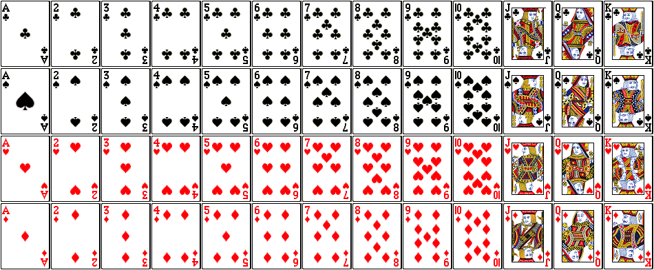
image credit: http://www.milefoot.com/math/discrete/counting/images/cards.png
Compute the probability of randomly drawing one card from a deck and getting an Ace.
Solution
There are 52 cards in the deck and 4 Aces.
Thus, \(P(\text{Ace})=\dfrac{4}{52}=\dfrac{1}{13} \approx 0.0769 \).
We can also think of probabilities as percents: There is a 7.69% chance that a randomly selected card will be an Ace.
Draw a single card from a well shuffled deck of 52 cards. Find the following probabilities:
- \(P(\text{red})\)
- \(P(\text{heart})\)
- \(P(\text{red 5})\)
- Answer
-
- \(P(\text{red}) = \dfrac{ \text {number of red cards}}{\text { total number of cards }} = \dfrac{26}{52} = \dfrac{1}{2}\). The probability that the card is red is \(\dfrac{1}{2}\).
- \(P(\text{heart}) = \dfrac{ \text {number of hearts}}{\text { total number of cards }} = \dfrac{13}{52} = \dfrac{1}{4}\). The probability that the card is a heart is \(\dfrac{1}{4}\).
- \(P(\text{red 5}) = \dfrac{ \text {number of red fives}}{\text { total number of cards }} = \dfrac{2}{52} = \dfrac{1}{26}\). The probability that the card is a red five is \(\dfrac{1}{26}\).
Law of Large Numbers
When studying probabilities, many times the law of large numbers will apply. If you want to observe what the probability is of getting tails when flipping a coin, you could do an experiment. Suppose you flip a coin 20 times and the coin comes up tails 9 times. Then, using an empirical probability, the probability of getting tails is \(\dfrac{9}{20}\) = 45%. However, we know that the theoretical probability for getting tails should be \(\dfrac{1}{2}\) = 50%. Why is this different? It is because there is error inherent to sampling methods. However, if you flip the coin 100 times or 1000 times, and use the information to calculate an empirical probability for getting tails, then the probabilities you will observe will become closer to the theoretical probability of 50%. This is the law of large numbers. The study of statistics involves looking at data (such as "tails come up 9 times in 20 tosses" and relating to the theoretical probabilities.
The law of large numbers says that as the number of times an experiment is repeated increases, the observed empirical probability of an event will approach the calculated theoretical probability of the same event.