8.5: Box Plots

Last updated
Save as PDF

Page ID: 121066

David Lippman & Jeff Eldridge
Pierce College via The OpenTextBookStore

$ \newcommand{\vecs}[1]{\overset { \scriptstyle \rightharpoonup} {\mathbf{#1}} } $ $ \newcommand{\vecd}[1]{\overset{-\!-\!\rightharpoonup}{\vphantom{a}\smash {#1}}} $$\newcommand{\id}{\mathrm{id}}$ $ \newcommand{\Span}{\mathrm{span}}$ $ \newcommand{\kernel}{\mathrm{null}\,}$ $ \newcommand{\range}{\mathrm{range}\,}$ $ \newcommand{\RealPart}{\mathrm{Re}}$ $ \newcommand{\ImaginaryPart}{\mathrm{Im}}$ $ \newcommand{\Argument}{\mathrm{Arg}}$ $ \newcommand{\norm}[1]{\| #1 \|}$ $ \newcommand{\inner}[2]{\langle #1, #2 \rangle}$ $ \newcommand{\Span}{\mathrm{span}}$ $\newcommand{\id}{\mathrm{id}}$ $ \newcommand{\Span}{\mathrm{span}}$ $ \newcommand{\kernel}{\mathrm{null}\,}$ $ \newcommand{\range}{\mathrm{range}\,}$ $ \newcommand{\RealPart}{\mathrm{Re}}$ $ \newcommand{\ImaginaryPart}{\mathrm{Im}}$ $ \newcommand{\Argument}{\mathrm{Arg}}$ $ \newcommand{\norm}[1]{\| #1 \|}$ $ \newcommand{\inner}[2]{\langle #1, #2 \rangle}$ $ \newcommand{\Span}{\mathrm{span}}$$\newcommand{\AA}{\unicode[.8,0]{x212B}}$

Learning Objectives

Find the 5-number summary of a data set
Construct and interpret a box plot for a data set

5-Number Summary

While quartiles are not a 1-number summary of spread like standard deviation, the quartiles are used with the median, minimum, and maximum values to form a 5-number summary of the data.

5-Number Summary

The 5-number summary takes the form:

Minimum, $Q_1$, Median, $Q_3$, Maximum

The 5-number summary is written as a list of numbers. It is understood by context what each value in the list represents.

Example $\PageIndex{1}$

Find the 5-number summaries for the 9 female sample and the 8 female sample from the previous section.

59 60 62 64 66 67 69 70 72

59 60 62 64 66 67 69 70

Solution

For the 9 female sample, the median is 66, the minimum is 59, and the maximum is 72. The 5-number summary is: 59, 61, 66, 69.5, 72.

For the 8 female sample, the median is 65, the minimum is 59, and the maximum is 70, so the 5-number summary would be: 59, 61, 65, 68, 70.

Example $\PageIndex{2}$

Find the 5-number summary of the quiz score data from the previous section.

section A: 5 5 5 5 5 5 5 5 5 5
section B: 0 0 0 0 0 10 10 10 10 10
section C: 4 4 4 5 5 5 5 6 6 6
section D: 0 5 5 5 5 5 5 5 5 10

Solution

In each section, the median is the average of 5^th and 6^th data values. The first quartile is the 3^rd data value, and the third quartile is the 8^th data value. Creating the 5-number summaries:

$\begin{array}{|l|l|}
\hline \text { section and data } & \text { 5-number summary } \\
\hline \text { section A: 5 5 5 5 5 5 5 5 5 5 } & 5,5,5,5,5 \\
\hline \text { section B: 0 0 0 0 0 10 10 10 10 10 } & 0,0,5,10,10 \\
\hline \text { section C: 4 4 4 5 5 5 5 6 6 6 } & 4,4,5,6,6 \\
\hline \text { section D: 0 5 5 5 5 5 5 5 5 10 } & 0,5,5,5,10 \\
\hline
\end{array}$

Of course, with a relatively small data set, finding a 5-number summary is a bit silly, since the summary contains almost as many values as the original data.

Try It $\PageIndex{1}$

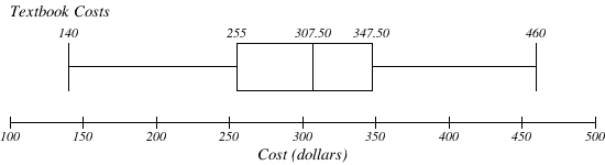
The total cost of textbooks for the term was collected from 36 students. Find the 5-number summary of this data.

$140 $160 $160 $165 $180 $220 $235 $240 $250 $260 $280 $285

$285 $285 $290 $300 $300 $305 $310 $310 $315 $315 $320 $320

$330 $340 $345 $350 $355 $360 $360 $380 $395 $420 $460 $460

Answer

The data is already in order, so we don’t need to sort it first.

The minimum value is $140 and the maximum is $460.

There are 36 data values so $n=36 .$ 36 is an even number, so the median is the average of the $18^{\text {th }}$ and $19^{\text {th }}$ data values, $\$ 305$ and $\$ 310$. The median is $\$ 307.50$

To find the first quartile, the number of data in the first half is $n = 18.$ Since 18 is an even number, we know $\mathrm{Q}_{1}$ is the average of the $9^{\text {th }}$ and $10^{\text {th }}$ data values, $\$ 250$ and $\$ 260 . \mathrm{Q}_{1}=$ $\$ 255$

To find the third quartile, the number of data in the second half is also $n = 18.$ Since 18 is an even number, we know $\mathrm{Q}_{3}$ is the average of the $9^{\text {th }}$ and $10^{\text {th }}$ data values of the second half of the data set (or the 18 + 9 = 27^th and 28^th data values in the original data set), $\$ 345$ and $\$ 350$. $\mathrm{Q}_{3}=\$ 347.50$

The 5-number summary of this data is: $140, $255, $307.50, $347.50, $460

Example $\PageIndex{3}$

Returning to the household income data from earlier, find the 5-number summary.

$\begin{array}{|l|l|}
\hline \textbf { Income (thousands of dollars) } & \textbf { Frequency } \\
\hline 15 & 6 \\
\hline 20 & 8 \\
\hline 25 & 11 \\
\hline 30 & 17 \\
\hline 35 & 19 \\
\hline 40 & 20 \\
\hline 45 & 12 \\
\hline 50 & 7 \\
\hline
\end{array}$

Solution

By adding the frequencies, we can see there are $n$ = 100 data values represented in the table. In a previous example, we found the median was the mean of the 50^th and 51^st data values, $35 thousand. We can see in the table that the minimum income is $15 thousand, and the maximum is $50 thousand.

To find $Q_1$, we find the median of the first 50 data values. It will be the mean of the 25^th and 26^th data values.

Counting up in the data as we did before,

$\begin{array}{ll} \text{There are 6 data values of \$15, so} & \text{values 1 to 6 are \$15 thousand} \\ \text{The next 8 data values are \$20, so} & \text{values 7 to (6 + 8) = 14 are \$20 thousand} \\ \text{The next 11 data values are \$25, so} & \text{values 15 to (14 + 11) = 25 are \$25 thousand} \\ \text{The next 17 data values are \$30, so} & \text{values 26 to (25 + 17) = 42 are \$30 thousand} \end{array}$

The 25^th data value is $25 thousand, and the 26^th data value is $30 thousand, so $Q_1$ will be the mean of these: $\dfrac{(25 + 30)}{2} = \$27.5$ thousand.

To find $Q_3$, we find the median of the second 50 data values. It will be the mean of the 75^th and 76^th data values. Continuing our counting from earlier,

$\begin{array}{ll} \text{The next 19 data values are \$35, so} & \text{values 43 to (42 + 19) = 61 are \$35 thousand} \\ \text{The next 20 data values are \$40, so} & \text{values 61 to (61 + 20) = 81 are \$40 thousand} \end{array}$

Both the 75^th and 76^th data values lie in this group, so $Q_3$ will be $40 thousand.

Putting these values together into a 5-number summary, we get: 15, 27.5, 35, 40, 50 (in thousands of dollars).

Note that the 5 number summary divides the data into four intervals, each of which will contain about 25% of the data. In the previous example, that means about 25% of households have income between $40 thousand and $50 thousand.

Box Plots

For visualizing data, there is a graphical representation of a 5-number summary called a box plot, or box-and-whisker graph.

Box plot

A box plot is a graphical representation of a 5-number summary.

To create a box plot, a scaled number line is first drawn. A box is drawn from the first quartile to the third quartile, and a line is drawn through the box at the median. “Whiskers” are extended out to the minimum and maximum values. Be sure to give the graph a title and label the number line.

Example $\PageIndex{4}$

Construct a box plot for the household income data.

Solution

The box plot below is based on the household income data with 5-number summary: 15, 27.5, 35, 40, 50

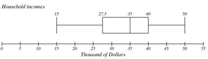
A boxplot titled Household incomes. The horizontal axis is labeled Thousands of dollars and goes from 0 to 55 with scale of 5. There is a box drawn from 27.5 to 40, with a vertical line dividing it at 35. From the box, a line extends out to the left to 15 where there's a vertical line, and from the box a line extends out to the right to 50 where there's a vertical line.

The box plot illustrates how spread or concentrated the data is. Since each part of the box plot represents a quarter of the data set, we can see that the data in the first quarter is more spread out, but the data between the second and third quartiles is more concentrated. There are the same number of data values in each part: 25 values between $15 to $27.5, 25 values between $27.5 to $35 thousand, 25 values between $35 to $40 thousand and 25 values between $40 to $50 thousand.

Try It $\PageIndex{2}$

Create a box plot based on the textbook price data from the last Try It.

Answer

Box plots are particularly useful for comparing data from two populations.

Example $\PageIndex{5}$

The box plots of service times for two fast-food restaurants are shown below. Discuss the differences between the stores based on the box plots.

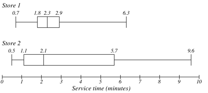
A comparative boxplot. The horizontal axis is labeled service times (minutes) and goes from 0 to 10. The first box labeled Store 1 has a box from 1.8 to 2.9 with a middle division at 2.3, and whiskers out to 0.7 and 6.3. The second box labeled Store 2 has a box from 1.1 to 5.7 with a middle division at 2.1, and whiskers out to 0.5 and 9.6.

Solution

While store 2 had a slightly shorter median service time (2.1 minutes vs. 2.3 minutes), store 2 is less consistent, with a wider spread of the data.

At store 1, 75% of customers were served within 2.9 minutes, while at store 2, 75% of customers were served within 5.7 minutes.

Which store should you go to in a hurry? That depends upon your opinions about luck: 25% of customers at store 2 had to wait between 5.7 and 9.6 minutes!

Try It $\PageIndex{3}$

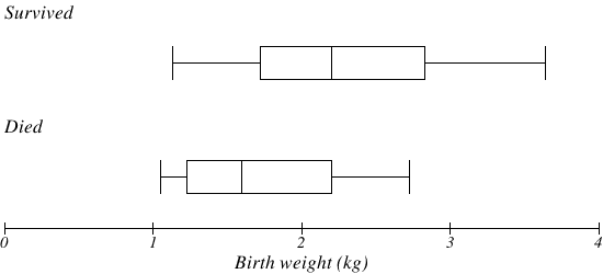
The box plot below is based on the birth weights in kilograms of infants with severe idiopathic respiratory distress syndrome (SIRDS) [1]. There are separate box plots to show the birth weights of infants who survived and those that did not. Compare and contrast the groups based on the box plots.

A comparative boxplot. The horizontal axis is labeled Birth weight (kg) and goes from 0 to 4. The box values are not labeled, so approximates are given here. The first box labeled Survived has a box from 1.6 to 2.7 with a middle division at 2.2, and whiskers out to 1.2 and 3.7. The second box labeled Died has a box from 1.3 to 2.2 with a middle division at 1.5, and whiskers out to 1.1 and 2.6.

Answer

Comparing the two groups, the box plots reveal that the birth weights of the infants that died appear to be, overall, less than the weights of infants that survived. In fact, we can see that the median birth weight of infants that survived is the same as the third quartile of the infants that died.

Similarly, we can see that the first quartile of the survivors is greater than the median weight of those that died, meaning that over 75% of the survivors had a birth weight greater than the median birth weight of those that died.

Looking at the maximum value for those that died and the third quartile of the survivors, we can see that over 25% of the survivors had birth weights greater than the heaviest infant that died.

The box plots give us a quick, albeit informal, way to determine that birth weight is quite likely linked to survival of infants with SIRDS.

[1] van Vliet, P.K. and Gupta, J.M. (1973) Sodium bicarbonate in idiopathic respiratory distress syndrome. Arch. Disease in Childhood, 48, 249–255. As quoted on http://openlearn.open.ac.uk/mod/ouco...&section=1.1

Search

5-Number Summary

Example \(\PageIndex{1}\)

Solution

Example \(\PageIndex{2}\)

Solution

Try It \(\PageIndex{1}\)

Example \(\PageIndex{3}\)

Solution

Box plot

Example \(\PageIndex{4}\)

Solution

Try It \(\PageIndex{2}\)

Example \(\PageIndex{5}\)

Solution

Try It \(\PageIndex{3}\)