
Stokes' Theorem
- Page ID
- 21061

\( \newcommand{\vecs}[1]{\overset { \scriptstyle \rightharpoonup} {\mathbf{#1}} } \)
\( \newcommand{\vecd}[1]{\overset{-\!-\!\rightharpoonup}{\vphantom{a}\smash {#1}}} \)
\( \newcommand{\dsum}{\displaystyle\sum\limits} \)
\( \newcommand{\dint}{\displaystyle\int\limits} \)
\( \newcommand{\dlim}{\displaystyle\lim\limits} \)
\( \newcommand{\id}{\mathrm{id}}\) \( \newcommand{\Span}{\mathrm{span}}\)
( \newcommand{\kernel}{\mathrm{null}\,}\) \( \newcommand{\range}{\mathrm{range}\,}\)
\( \newcommand{\RealPart}{\mathrm{Re}}\) \( \newcommand{\ImaginaryPart}{\mathrm{Im}}\)
\( \newcommand{\Argument}{\mathrm{Arg}}\) \( \newcommand{\norm}[1]{\| #1 \|}\)
\( \newcommand{\inner}[2]{\langle #1, #2 \rangle}\)
\( \newcommand{\Span}{\mathrm{span}}\)
\( \newcommand{\id}{\mathrm{id}}\)
\( \newcommand{\Span}{\mathrm{span}}\)
\( \newcommand{\kernel}{\mathrm{null}\,}\)
\( \newcommand{\range}{\mathrm{range}\,}\)
\( \newcommand{\RealPart}{\mathrm{Re}}\)
\( \newcommand{\ImaginaryPart}{\mathrm{Im}}\)
\( \newcommand{\Argument}{\mathrm{Arg}}\)
\( \newcommand{\norm}[1]{\| #1 \|}\)
\( \newcommand{\inner}[2]{\langle #1, #2 \rangle}\)
\( \newcommand{\Span}{\mathrm{span}}\) \( \newcommand{\AA}{\unicode[.8,0]{x212B}}\)
\( \newcommand{\vectorA}[1]{\vec{#1}} % arrow\)
\( \newcommand{\vectorAt}[1]{\vec{\text{#1}}} % arrow\)
\( \newcommand{\vectorB}[1]{\overset { \scriptstyle \rightharpoonup} {\mathbf{#1}} } \)
\( \newcommand{\vectorC}[1]{\textbf{#1}} \)
\( \newcommand{\vectorD}[1]{\overrightarrow{#1}} \)
\( \newcommand{\vectorDt}[1]{\overrightarrow{\text{#1}}} \)
\( \newcommand{\vectE}[1]{\overset{-\!-\!\rightharpoonup}{\vphantom{a}\smash{\mathbf {#1}}}} \)
\( \newcommand{\vecs}[1]{\overset { \scriptstyle \rightharpoonup} {\mathbf{#1}} } \)
\(\newcommand{\longvect}{\overrightarrow}\)
\( \newcommand{\vecd}[1]{\overset{-\!-\!\rightharpoonup}{\vphantom{a}\smash {#1}}} \)
\(\newcommand{\avec}{\mathbf a}\) \(\newcommand{\bvec}{\mathbf b}\) \(\newcommand{\cvec}{\mathbf c}\) \(\newcommand{\dvec}{\mathbf d}\) \(\newcommand{\dtil}{\widetilde{\mathbf d}}\) \(\newcommand{\evec}{\mathbf e}\) \(\newcommand{\fvec}{\mathbf f}\) \(\newcommand{\nvec}{\mathbf n}\) \(\newcommand{\pvec}{\mathbf p}\) \(\newcommand{\qvec}{\mathbf q}\) \(\newcommand{\svec}{\mathbf s}\) \(\newcommand{\tvec}{\mathbf t}\) \(\newcommand{\uvec}{\mathbf u}\) \(\newcommand{\vvec}{\mathbf v}\) \(\newcommand{\wvec}{\mathbf w}\) \(\newcommand{\xvec}{\mathbf x}\) \(\newcommand{\yvec}{\mathbf y}\) \(\newcommand{\zvec}{\mathbf z}\) \(\newcommand{\rvec}{\mathbf r}\) \(\newcommand{\mvec}{\mathbf m}\) \(\newcommand{\zerovec}{\mathbf 0}\) \(\newcommand{\onevec}{\mathbf 1}\) \(\newcommand{\real}{\mathbb R}\) \(\newcommand{\twovec}[2]{\left[\begin{array}{r}#1 \\ #2 \end{array}\right]}\) \(\newcommand{\ctwovec}[2]{\left[\begin{array}{c}#1 \\ #2 \end{array}\right]}\) \(\newcommand{\threevec}[3]{\left[\begin{array}{r}#1 \\ #2 \\ #3 \end{array}\right]}\) \(\newcommand{\cthreevec}[3]{\left[\begin{array}{c}#1 \\ #2 \\ #3 \end{array}\right]}\) \(\newcommand{\fourvec}[4]{\left[\begin{array}{r}#1 \\ #2 \\ #3 \\ #4 \end{array}\right]}\) \(\newcommand{\cfourvec}[4]{\left[\begin{array}{c}#1 \\ #2 \\ #3 \\ #4 \end{array}\right]}\) \(\newcommand{\fivevec}[5]{\left[\begin{array}{r}#1 \\ #2 \\ #3 \\ #4 \\ #5 \\ \end{array}\right]}\) \(\newcommand{\cfivevec}[5]{\left[\begin{array}{c}#1 \\ #2 \\ #3 \\ #4 \\ #5 \\ \end{array}\right]}\) \(\newcommand{\mattwo}[4]{\left[\begin{array}{rr}#1 \amp #2 \\ #3 \amp #4 \\ \end{array}\right]}\) \(\newcommand{\laspan}[1]{\text{Span}\{#1\}}\) \(\newcommand{\bcal}{\cal B}\) \(\newcommand{\ccal}{\cal C}\) \(\newcommand{\scal}{\cal S}\) \(\newcommand{\wcal}{\cal W}\) \(\newcommand{\ecal}{\cal E}\) \(\newcommand{\coords}[2]{\left\{#1\right\}_{#2}}\) \(\newcommand{\gray}[1]{\color{gray}{#1}}\) \(\newcommand{\lgray}[1]{\color{lightgray}{#1}}\) \(\newcommand{\rank}{\operatorname{rank}}\) \(\newcommand{\row}{\text{Row}}\) \(\newcommand{\col}{\text{Col}}\) \(\renewcommand{\row}{\text{Row}}\) \(\newcommand{\nul}{\text{Nul}}\) \(\newcommand{\var}{\text{Var}}\) \(\newcommand{\corr}{\text{corr}}\) \(\newcommand{\len}[1]{\left|#1\right|}\) \(\newcommand{\bbar}{\overline{\bvec}}\) \(\newcommand{\bhat}{\widehat{\bvec}}\) \(\newcommand{\bperp}{\bvec^\perp}\) \(\newcommand{\xhat}{\widehat{\xvec}}\) \(\newcommand{\vhat}{\widehat{\vvec}}\) \(\newcommand{\uhat}{\widehat{\uvec}}\) \(\newcommand{\what}{\widehat{\wvec}}\) \(\newcommand{\Sighat}{\widehat{\Sigma}}\) \(\newcommand{\lt}{<}\) \(\newcommand{\gt}{>}\) \(\newcommand{\amp}{&}\) \(\definecolor{fillinmathshade}{gray}{0.9}\)- Explain the meaning of Stokes’ theorem.
- Use Stokes’ theorem to evaluate a line integral.
- Use Stokes’ theorem to calculate a surface integral.
- Use Stokes’ theorem to calculate a curl.
In this section, we study Stokes’ theorem, a higher-dimensional generalization of Green’s theorem. This theorem, like the Fundamental Theorem for Line Integrals and Green’s theorem, is a generalization of the Fundamental Theorem of Calculus to higher dimensions. Stokes’ theorem relates a vector surface integral over surface \(S\) in space to a line integral around the boundary of \(S\). Therefore, just as the theorems before it, Stokes’ theorem can be used to reduce an integral over a geometric object \(S\) to an integral over the boundary of \(S\). In addition to allowing us to translate between line integrals and surface integrals, Stokes’ theorem connects the concepts of curl and circulation. Furthermore, the theorem has applications in fluid mechanics and electromagnetism. We use Stokes’ theorem to derive Faraday’s law, an important result involving electric fields.
Stokes’ Theorem
Stokes’ theorem says we can calculate the flux of \( curl \,\vecs{F}\) across surface \(S\) by knowing information only about the values of \(\vecs{F}\) along the boundary of \(S\). Conversely, we can calculate the line integral of vector field \(\vecs{F}\) along the boundary of surface \(S\) by translating to a double integral of the curl of \(\vecs{F}\) over \(S\).
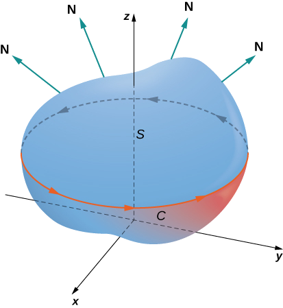
Let \(S\) be an oriented smooth surface with unit normal vector \(\vecs{N}\). Furthermore, suppose the boundary of \(S\) is a simple closed curve \(C\). The orientation of \(S\) induces the positive orientation of \(C\) if, as you walk in the positive direction around \(C\) with your head pointing in the direction of \(\vecs{N}\), the surface is always on your left. With this definition in place, we can state Stokes’ theorem.
Let \(S\) be a piecewise smooth oriented surface with a boundary that is a simple closed curve \(C\) with positive orientation (Figure \(\PageIndex{1}\)). If \(\vecs{F}\) is a vector field with component functions that have continuous partial derivatives on an open region containing \(S\), then
\[\int_C \vecs{F} \cdot d \vecs{r} = \iint_S curl \, \vecs{F} \cdot d\vecs S. \label{Stokes1} \]
Suppose surface \(S\) is a flat region in the \(xy\)-plane with upward orientation. Then the unit normal vector is \(\vecs{k}\) and surface integral
\[\iint_S curl \, \vecs{F} \cdot d\vecs{S} \nonumber \]
is actually the double integral
\[\iint_S curl \, \vecs{F} \cdot \vecs{k} \, dA. \nonumber \]
In this special case, Stokes’ theorem gives
\[\int_C \vecs{F} \cdot d\vecs{r} = \iint_S curl \, \vecs{F} \cdot \vecs{k} \, dA. \nonumber \]
However, this is the flux form of Green’s theorem, which shows us that Green’s theorem is a special case of Stokes’ theorem. Green’s theorem can only handle surfaces in a plane, but Stokes’ theorem can handle surfaces in a plane or in space.
The complete proof of Stokes’ theorem is beyond the scope of this text. We look at an intuitive explanation for the truth of the theorem and then see proof of the theorem in the special case that surface \(S\) is a portion of a graph of a function, and \(S\), the boundary of \(S\), and \(\vecs{F}\) are all fairly tame.
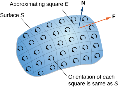
First, we look at an informal proof of the theorem. This proof is not rigorous, but it is meant to give a general feeling for why the theorem is true. Let \(S\) be a surface and let \(D\) be a small piece of the surface so that \(D\) does not share any points with the boundary of \(S\). We choose \(D\) to be small enough so that it can be approximated by an oriented square \(E\). Let \(D\) inherit its orientation from \(S\), and give \(E\) the same orientation. This square has four sides; denote them \(E_l, \, E_r, \, E_u\), and \(E_d\) for the left, right, up, and down sides, respectively. On the square, we can use the flux form of Green’s theorem:
\[\int_{E_l+E_d+E_r+E_u} \vecs{F} \cdot d \vecs{r} = \iint_E curl \, \vecs{F} \cdot \vecs{N} \, d \vecs{S} = \iint_E curl \, \vecs{F} \cdot d\vecs{S}. \nonumber \]
To approximate the flux over the entire surface, we add the values of the flux on the small squares approximating small pieces of the surface (Figure \(\PageIndex{2}\)).
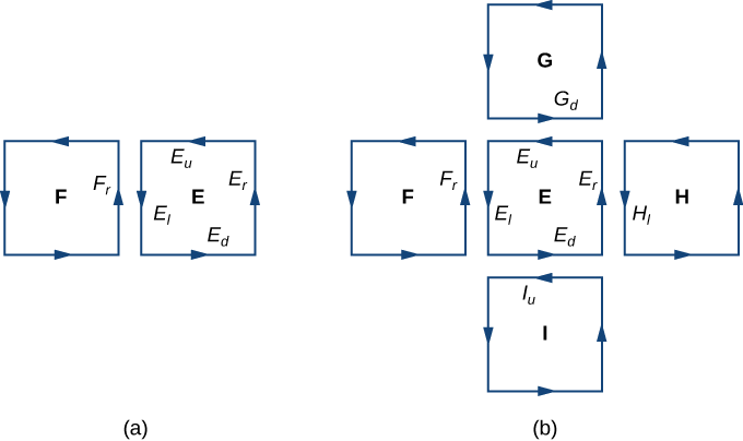
By Green’s theorem, the flux across each approximating square is a line integral over its boundary. Let \(F\) be an approximating square with an orientation inherited from \(S\) and with a right side \(E_l\) (so \(F\) is to the left of \(E\)). Let \(F_r\) denote the right side of \(F\); then, \(E_l = - F_r\). In other words, the right side of \(F\) is the same curve as the left side of \(E\), just oriented in the opposite direction. Therefore,
\[\int_{E_l} \vecs F \cdot d\vecs r = - \int_{F_r} \vecs F \cdot d\vecs r. \nonumber \]
As we add up all the fluxes over all the squares approximating surface \(S\), line integrals
\[\int_{E_l} \vecs{F} \cdot d \vecs{r} \nonumber \]
and
\[ \int_{F_r} \vecs{F} \cdot d\vecs{r} \nonumber \]
cancel each other out. The same goes for the line integrals over the other three sides of \(E\). These three line integrals cancel out with the line integral of the lower side of the square above \(E\), the line integral over the left side of the square to the right of \(E\), and the line integral over the upper side of the square below \(E\) (Figure \(\PageIndex{3}\)). After all this cancelation occurs over all the approximating squares, the only line integrals that survive are the line integrals over sides approximating the boundary of \(S\). Therefore, the sum of all the fluxes (which, by Green’s theorem, is the sum of all the line integrals around the boundaries of approximating squares) can be approximated by a line integral over the boundary of \(S\). In the limit, as the areas of the approximating squares go to zero, this approximation gets arbitrarily close to the flux.
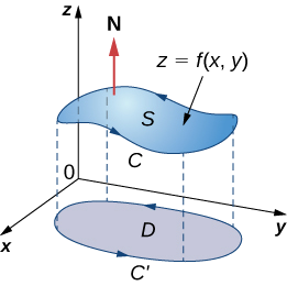
Let’s now look at a rigorous proof of the theorem in the special case that \(S\) is the graph of function \(z = f(x,y)\), where \(x\) and \(y\) vary over a bounded, simply connected region \(D\) of finite area (Figure \(\PageIndex{4}\)). Furthermore, assume that \(f\) has continuous second-order partial derivatives. Let \(C\) denote the boundary of \(S\) and let \(C'\) denote the boundary of \(D\). Then, \(D\) is the “shadow” of \(S\) in the plane and \(C'\) is the “shadow” of \(C\). Suppose that \(S\) is oriented upward. The counterclockwise orientation of \(C\) is positive, as is the counterclockwise orientation of \(C'\). Let \(\vecs F(x,y,z) = \langle P,Q,R \rangle\) be a vector field with component functions that have continuous partial derivatives.
We take the standard parameterization of \(S \, : \, x = x, \, y = y, \, z = g(x,y)\). The tangent vectors are \(\vecs t_x = \langle 1,0,g_x \rangle\) and \(\vecs t_y = \langle 0,1,g_y \rangle\), and therefore \(\vecs t_x \times \vecs t_y = \langle -g_x, \, -g_y, \, 1 \rangle\).
\[\iint_S curl \, \vecs{F} \cdot d\vecs{S} = \iint_D [- (R_y - Q_z)z_x - (P_z - R_x)z_y + (Q_x - P_y)] \, dA, \nonumber \]
where the partial derivatives are all evaluated at \((x,y,g(x,y))\), making the integrand depend on \(x\) and \(y\) only. Suppose \(\langle x (t), \, y(t) \rangle, \, a \leq t \leq b\) is a parameterization of \(C'\). Then, a parameterization of \(C\) is \(\langle x (t), \, y(t), \, g(x(t), \, y(t))\rangle, \, a \leq t \leq b\). Armed with these parameterizations, the Chain rule, and Green’s theorem, and keeping in mind that \(P\), \(Q\) and \(R\) are all functions of \(x\) and \(y\), we can evaluate line integral
\[ \begin{align*} \int_C \vecs{F} \cdot d \vecs{r} &= \int_a^b (Px'(t) + Qy'(t) + Rz'(t)) \, dt \\[4pt] &= \int_a^b \left[Px'(t) + Qy'(t) + R\left(\dfrac{\partial z}{\partial x} \dfrac{dx}{dt} + \dfrac{\partial z}{\partial y} \dfrac{dy}{dt}\right) \right] dt \\[4pt] &= \int_a^b \left[ \left(P + R \dfrac{\partial z}{\partial x} \right) x' (t) + \left(Q + R \dfrac{\partial z}{\partial y} \right) y'(t) \right] dt \\[4pt] &= \int_{C'} \left(P + R \dfrac{\partial z}{\partial x} \right)\, dx + \left(Q + R \dfrac{\partial z}{\partial y} \right) \, dy \\[4pt] &= \iint_D \left[ \dfrac{\partial}{\partial x} \left( Q + R \dfrac{\partial z}{\partial y} \right) - \dfrac{\partial}{\partial y} \left(P + R \dfrac{\partial z}{\partial x} \right) \right] \, dA \\[4pt] &=\iint_D \left(\dfrac{\partial Q}{\partial x} + \dfrac{\partial Q}{\partial z} \dfrac{\partial z}{\partial x} + \dfrac{\partial R}{\partial x} \dfrac{\partial z}{\partial y} + \dfrac{\partial R}{\partial z}\dfrac{\partial z}{\partial x} \dfrac{\partial z}{\partial y} + R \dfrac{\partial^2 z}{\partial x \partial y} \right) - \left(\dfrac{\partial P}{\partial y} + \dfrac{\partial P}{\partial z} \dfrac{\partial z}{\partial y} + \dfrac{\partial R}{\partial z} \dfrac{\partial z}{\partial y} \dfrac{\partial z}{\partial x} + R \dfrac{\partial^2 z}{\partial y \partial x} \right) \end{align*} \nonumber \]
By Clairaut’s theorem,
\[\dfrac{\partial^2 z}{\partial x \partial y} = \dfrac{\partial^2 z}{\partial y \partial x} \nonumber \]
Therefore, four of the terms disappear from this double integral, and we are left with
\[\iint_D [- (R_y - Q_z)Z_x - (P_z - R_x) z_y + (Q_x - P_y)] \, dA, \nonumber \]
which equals
\[\iint_S curl \, \vecs{F} \cdot d\vecs{S}. \nonumber \]
\(\Box\)
We have shown that Stokes’ theorem is true in the case of a function with a domain that is a simply connected region of finite area. We can quickly confirm this theorem for another important case: when vector field \(\vecs{F}\) is a conservative field. If \(\vecs{F}\) is conservative, the curl of \(\vecs{F}\) is zero, so
\[\iint_S curl \, \vecs{F} \cdot d\vecs{S} = 0. \nonumber \]
Since the boundary of \(S\) is a closed curve, the integral
\[\int_C \vecs{F} \cdot d\vecs{r}. \nonumber \]
is also zero.
Verify that Stokes’ theorem is true for vector field \(\vecs{F}(x,y) = \langle -z,x,0 \rangle\) and surface \(S\), where \(S\) is the hemisphere, oriented outward, with parameterization \(\vecs r(\phi, \theta) = \langle \sin \phi \, \cos \theta, \, \sin \phi \, \sin \theta, \, \cos \phi \rangle, \, 0 \leq \theta \leq \pi, \, 0 \leq \phi \leq \pi\) as shown in Figure \(\PageIndex{5}\).
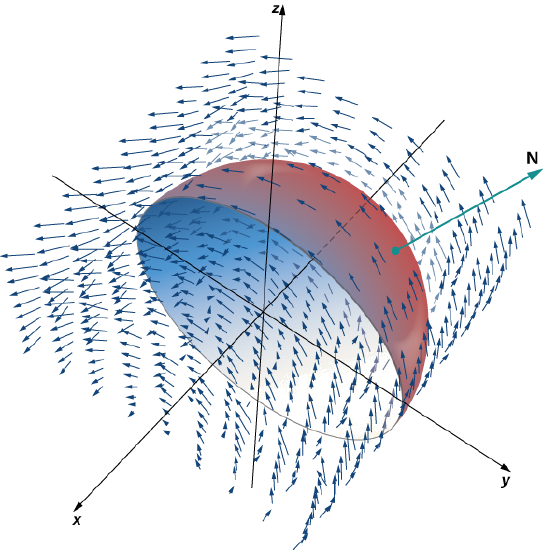
Solution
Let \(C\) be the boundary of \(S\). Note that \(C\) is a circle of radius 1, centered at the origin, sitting in plane \(y = 0\). This circle has parameterization \(\langle \cos t, \, 0, \, \sin t \rangle, \, 0 \leq t \leq 2\pi\). the equation for scalar surface integrals
\[ \begin{align*} \int_C \vecs{F} \cdot d \vecs{r} &= \int_0^{2\pi} \langle -\sin t, \, \cos t, \, 0 \rangle \cdot \langle - \sin t, \, 0, \, \cos t \rangle \, dt \\[4pt] &= \int_0^{2\pi} \sin^2 t \, dt \\[4pt] &= \pi. \end{align*}\]
By the equation for vector line integrals,
\[ \begin{align*} \iint_S \, curl \, \vecs{F} \cdot d\vecs S &= \iint_D curl \, \vecs{F} (\vecs r (\phi,\theta)) \cdot ( \vecs t_{\phi} \times \vecs t_{\theta}) \, dA \\[4pt] &= \iint_D \langle 0, -1, 1 \rangle \cdot \langle \cos \theta \, \sin^2 \phi, \, \sin \theta \, \sin^2 \phi, \, \sin \phi \, \cos \phi \rangle \, dA \\[4pt] &= \int_0^{\pi} \int_0^{\pi} (\sin \phi \, \cos \phi - \sin \theta \, \sin^2 \phi ) \, d\phi d\theta \\[4pt] &= \dfrac{\pi}{2} \int_0^{\pi} \sin \theta \, d\theta \\[4pt] &= \pi.\end{align*}\]
Therefore, we have verified Stokes’ theorem for this example.
Verify that Stokes’ theorem is true for vector field \(\vecs{F}(x,y,z) = \langle y,x,-z \rangle \) and surface \(S\), where \(S\) is the upwardly oriented portion of the graph of \(f(x,y) = x^2 y\) over a triangle in the \(xy\)-plane with vertices \((0,0), \, (2,0)\), and \((0,2)\).
- Hint
-
Calculate the double integral and line integral separately.
- Answer
-
Both integrals give \(-\dfrac{136}{45}\):
Calculate the line integral
\[\int_C \vecs{F} \cdot d\vecs{r}, \nonumber \]
where \(\vecs{F} = \langle xy, \, x^2 + y^2 + z^2, \, yz \rangle\) and \(C\) is the boundary of the parallelogram with vertices \((0,0,1), \, (0,1,0), \, (2,0,-1)\), and \((2,1,-2)\).
Solution
To calculate the line integral directly, we need to parameterize each side of the parallelogram separately, calculate four separate line integrals, and add the result. This is not overly complicated, but it is time-consuming.
By contrast, let’s calculate the line integral using Stokes’ theorem. Let \(S\) denote the surface of the parallelogram. Note that \(S\) is the portion of the graph of \(z = 1 - x - y\) for \((x,y)\) varying over the rectangular region with vertices \((0,0), \, (0,1), \, (2,0)\), and \((2,1)\) in the \(xy\)-plane. Therefore, a parameterization of \(S\) is \(\langle x,y, \, 1 - x - y \rangle, \, 0 \leq x \leq 2, \, 0 \leq y \leq 1\). The curl of \(\vecs{F}\) is \( \langle -z, \, 0, \, x \rangle\),and Stokes’ theorem and the equation for scalar surface integrals
\[ \begin{align*} \int_C \vecs{F} \cdot d\vecs{r} &= \iint_S curl \, \vecs{F} \cdot d\vecs{S} \\[4pt] &= \int_0^2 \int_0^1 curl \, \vecs{F} (x,y) \cdot (\vecs t_x \times \vecs t_y) \, dy\, dx \\[4pt] &= \int_0^2 \int_0^1 \langle - (1 - x - y), \, 0, \, x \rangle \cdot ( \langle 1, \, 0, -1 \rangle \times \langle 0, \, 1, \, -1 \rangle ) \, dy \,dx \\[4pt] &= \int_0^2 \int_0^1 \langle x + y - 1, \, 0, \, x \rangle \cdot \langle 1, 1, 1 \rangle \, dy \, dx \\[4pt] &= \int_0^2 \int_0^1 2x + y - 1 \, dy \, dx \\[4pt] &= 3.\end{align*} \nonumber \]
Use Stokes’ theorem to calculate line integral
\[\int_C \vecs{F} \cdot d\vecs{r}, \nonumber \]
where \(\vecs{F} = \langle z,x,y \rangle \) and \(C\) is the boundary of a triangle with vertices \((0,0,1), \, (3,0,-2)\), and \((0,1,2)\).
- Hint
-
This triangle lies in plane \(z = 1 - x + y\).
- Answer
-
\(\dfrac{3}{2}\)
Interpretation of Curl
In addition to translating between line integrals and flux integrals, Stokes’ theorem can be used to justify the physical interpretation of curl that we have learned. Here we investigate the relationship between curl and circulation, and we use Stokes’ theorem to state Faraday’s law—an important law in electricity and magnetism that relates the curl of an electric field to the rate of change of a magnetic field.
Recall that if \(C\) is a closed curve and \(\vecs{F}\) is a vector field defined on \(C\), then the circulation of \(\vecs{F}\) around \(C\) is line integral
\[\int_C \vecs{F} \cdot d\vecs{r}. \nonumber \]
If \(\vecs{F}\) represents the velocity field of a fluid in space, then the circulation measures the tendency of the fluid to move in the direction of \(C\).
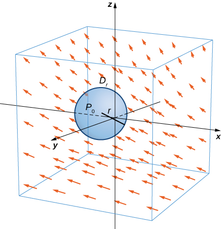
Let \(\vecs{F}\) be a continuous vector field and let \(D_{\tau}\) be a small disk of radius \(r\) with center \(P_0\) (Figure \(\PageIndex{7}\)). If \(D_{\tau}\) is small enough, then \((curl \, \vecs{F})(P) \approx (curl \, \vecs F)(P_0)\) for all points \(P\) in \(D_{\tau}\) because the curl is continuous. Let \(C_{\tau}\) be the boundary circle of \(D_{\tau}\): By Stokes’ theorem,
\[\int_{C_{\tau}} \vecs{F} \cdot d\vecs{r} = \iint_{D_{\tau}} curl \, \vecs{F} \cdot \vecs{N} \, d\vecs S \approx \iint_{D_{\tau}} (curl \, \vecs{F})(P_0) \cdot \vecs{N} (P_0) \, d\vecs S. \nonumber \]
The quantity \( (curl \, \vecs F)(P_0) \cdot \vecs N (P_0) \) is constant, and therefore
\[\iint_{D_{\tau}} (curl \, \vecs F)(P_0) \cdot \vecs N (P_0) \, d\vecs S = \pi r^2 [(curl \, \vecs F)(P_0) \cdot \vecs N (P_0)]. \nonumber \]
Thus
\[\int_{C_{\tau}} \vecs F \cdot d\vecs r \approx \pi r^2 [ (curl \, \vecs F)(P_0) \cdot \vecs N (P_0)], \nonumber \]
and the approximation gets arbitrarily close as the radius shrinks to zero. Therefore Stokes’ theorem implies that
\[(curl \, \vecs F)(P_0) \cdot \vecs N (P_0) = \lim_{r\rightarrow 0^+} \dfrac{1}{\pi r^2} \int_{C_{\tau}} \vecs F \cdot d\vecs r. \nonumber \]
This equation relates the curl of a vector field to the circulation. Since the area of the disk is \(\pi r^2\), this equation says we can view the curl (in the limit) as the circulation per unit area. Recall that if \(\vecs F\) is the velocity field of a fluid, then circulation \[\oint_{C_{\tau}} \vecs F \cdot d\vecs r = \oint_{C_{\tau}} \vecs F \cdot \vecs T \, ds \nonumber \] is a measure of the tendency of the fluid to move around \(C_{\tau}\): The reason for this is that \(\vecs F \cdot \vecs T\) is a component of \(\vecs F\) in the direction of \(\vecs T\), and the closer the direction of \(\vecs F\) is to \(\vecs T\), the larger the value of \(\vecs F \cdot \vecs T\) (remember that if \(\vecs a\) and \(\vecs b\) are vectors and \(\vecs b\) is fixed, then the dot product \(\vecs a \cdot \vecs b\) is maximal when \(\vecs a\) points in the same direction as \(\vecs b\)). Therefore, if \(\vecs F\) is the velocity field of a fluid, then \(curl \, \vecs F \cdot \vecs N\) is a measure of how the fluid rotates about axis \(\vecs N\). The effect of the curl is largest about the axis that points in the direction of \(\vecs N\), because in this case \(curl \, \vecs F \cdot \vecs N\) is as large as possible.
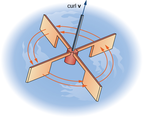
To see this effect in a more concrete fashion, imagine placing a tiny paddlewheel at point \(P_0\) (Figure \(\PageIndex{8}\)). The paddlewheel achieves its maximum speed when the axis of the wheel points in the direction of curl \(\vecs F\). This justifies the interpretation of the curl we have learned: curl is a measure of the rotation in the vector field about the axis that points in the direction of the normal vector \(\vecs N\), and Stokes’ theorem justifies this interpretation.
Now that we have learned about Stokes’ theorem, we can discuss applications in the area of electromagnetism. In particular, we examine how we can use Stokes’ theorem to translate between two equivalent forms of Faraday’s law. Before stating the two forms of Faraday’s law, we need some background terminology.
Let \(C\) be a closed curve that models a thin wire. In the context of electric fields, the wire may be moving over time, so we write \(C(t)\) to represent the wire. At a given time \(t\), curve \(C(t)\) may be different from original curve \(C\) because of the movement of the wire, but we assume that \(C(t)\) is a closed curve for all times \(t\). Let \(D(t)\) be a surface with \(C(t)\) as its boundary, and orient \(C(t)\) so that \(D(t)\) has positive orientation. Suppose that \(C(t)\)is in a magnetic field \(\vecs B(t)\) that can also change over time. In other words, \(\vecs{B}\) has the form
\[\vecs B(x,y,z) = \langle P(x,y,z), \, Q(x,y,z), \, R(x,y,z) \rangle, \nonumber \]
where \(P\), \(Q\), and \(R\) can all vary continuously over time. We can produce current along the wire by changing field \(\vecs B(t)\) (this is a consequence of Ampere’s law). Flux \(\displaystyle \phi (t) = \iint_{D(t)} \vecs B(t) \cdot d\vecs S\) creates electric field \(\vecs E(t)\) that does work. The integral form of Faraday’s law states that
\[Work = \int_{C(t)} \vecs E(t) \cdot d\vecs r = - \dfrac{\partial \phi}{\partial t}. \nonumber \]
In other words, the work done by \(\vecs{E}\) is the line integral around the boundary, which is also equal to the rate of change of the flux with respect to time. The differential form of Faraday’s law states that
\[curl \, \vecs{E} = - \dfrac{\partial \vecs B}{\partial t}. \nonumber \]
Using Stokes’ theorem, we can show that the differential form of Faraday’s law is a consequence of the integral form. By Stokes’ theorem, we can convert the line integral in the integral form into surface integral
\[-\dfrac{\partial \phi}{\partial t} = \int_{C(t)} \vecs E(t) \cdot d\vecs r = \iint_{D(t)} curl \,\vecs E(t) \cdot d\vecs S. \nonumber \]
Since \[\phi (t) = \iint_{D(t)} B(t) \cdot d\vecs S, \nonumber \] then as long as the integration of the surface does not vary with time we also have
\[- \dfrac{\partial \phi}{\partial t} = \iint_{D(t)} - \dfrac{\partial \vecs B}{\partial t} \cdot d\vecs S. \nonumber \]
Therefore,
\[\iint_{D(t)} - \dfrac{\partial \vecs B}{\partial t} \cdot d\vecs S = \iint_{D(t)} curl \,\vecs E \cdot d\vecs S. \nonumber \]
To derive the differential form of Faraday’s law, we would like to conclude that \(curl \,\vecs E = -\dfrac{\partial \vecs B}{\partial t}\): In general, the equation
\[\iint_{D(t)} - \dfrac{\partial \vecs B}{\partial t} \cdot d\vecs S = \iint_{D(t)} curl \,\vecs E \cdot d\vecs S \nonumber \]
is not enough to conclude that \(curl \, \vecs E = -\dfrac{\partial \vecs B}{\partial t}\): The integral symbols do not simply “cancel out,” leaving equality of the integrands. To see why the integral symbol does not just cancel out in general, consider the two single-variable integrals \(\displaystyle \int_0^1 x \, dx\) and \(\displaystyle \int_0^1 f(x)\, dx\), where
\[f(x) = \begin{cases}1, &\text{if } 0 \leq x \leq 1/2 \\ 0, & \text{if } 1/2 \leq x \leq 1. \end{cases} \nonumber \]
Both of these integrals equal \(\dfrac{1}{2}\), so \(\displaystyle \int_0^1 x \, dx = \int_0^1 f(x) \, dx\).
However, \(x \neq f(x)\). Analogously, with our equation \[\iint_{D(t)} - \dfrac{\partial \vecs B}{\partial t} \cdot d\vecs S = \iint_{D(t)} curl \, \vecs E \cdot d\vecs S, \nonumber \] we cannot simply conclude that \(curl \, \vecs E = -\dfrac{\partial \vecs B}{\partial t}\) just because their integrals are equal. However, in our context, equation
\[\iint_{D(t)} - \dfrac{\partial \vecs B}{\partial t} \cdot d\vecs S = \iint_{D(t)} curl \, \vecs E \cdot d\vecs S \nonumber \]
is true for any region, however small (this is in contrast to the single-variable integrals just discussed). If \(\vecs F\) and \(\vecs G\) are three-dimensional vector fields such that
\[\iint_S \vecs F \cdot d\vecs S = \iint_S \vecs G \cdot d\vecs S \nonumber \]
for any surface \(S\), then it is possible to show that \(\vecs F = \vecs G\) by shrinking the area of \(S\) to zero by taking a limit (the smaller the area of \(S\), the closer the value of \(\displaystyle \iint_S \vecs F \cdot d\vecs S\) to the value of \(\vecs F\) at a point inside \(S\)). Therefore, we can let area \(D(t)\) shrink to zero by taking a limit and obtain the differential form of Faraday’s law:
\[curl \,\vecs E = - \dfrac{\partial \vecs B}{\partial t}. \nonumber \]
In the context of electric fields, the curl of the electric field can be interpreted as the negative of the rate of change of the corresponding magnetic field with respect to time.
Calculate the curl of electric field \(\vecs{E}\) if the corresponding magnetic field is constant field \(\vecs B(t) = \langle 1, -4, 2 \rangle\).
Solution
Since the magnetic field does not change with respect to time, \(-\dfrac{\partial \vecs B}{\partial t} = \vecs 0\). By Faraday’s law, the curl of the electric field is therefore also zero.
AnalysisA consequence of Faraday’s law is that the curl of the electric field corresponding to a constant magnetic field is always zero.
Calculate the curl of electric field \(\vecs{E}\) if the corresponding magnetic field is \(\vecs B(t) = \langle tx, \, ty, \, -2tz \rangle, \, 0 \leq t < \infty.\)
- Hint
-
- Use the differential form of Faraday’s law.
- Notice that the curl of the electric field does not change over time, although the magnetic field does change over time.
- Answer
-
\(curl \, \vecs{E} = \langle x, \, y, \, -2z \rangle\)
Key Concepts
- Stokes’ theorem relates a flux integral over a surface to a line integral around the boundary of the surface. Stokes’ theorem is a higher dimensional version of Green’s theorem, and therefore is another version of the Fundamental Theorem of Calculus in higher dimensions.
- Stokes’ theorem can be used to transform a difficult surface integral into an easier line integral, or a difficult line integral into an easier surface integral.
- Through Stokes’ theorem, line integrals can be evaluated using the simplest surface with boundary \(C\).
- Faraday’s law relates the curl of an electric field to the rate of change of the corresponding magnetic field. Stokes’ theorem can be used to derive Faraday’s law.
Key Equations
- Stokes’ theorem
\[\int_C \vecs{F} \cdot d\vecs{r} = \iint_S curl \, \vecs{F} \cdot d\vecs{S} \nonumber \]
Glossary
- Stokes’ theorem
- relates the flux integral over a surface \(S\) to a line integral around the boundary \(C\) of the surface \(S\)
- surface independent
- flux integrals of curl vector fields are surface independent if their evaluation does not depend on the surface but only on the boundary of the surface
Applying Stokes’ Theorem
Stokes’ theorem translates between the flux integral of surface \(S\) to a line integral around the boundary of \(S\). Therefore, the theorem allows us to compute surface integrals or line integrals that would ordinarily be quite difficult by translating the line integral into a surface integral or vice versa. We now study some examples of each kind of translation.
Example \(\PageIndex{2}\): Calculating a Surface Integral
Calculate surface integral
\[\iint_S curl \, \vecs{F} \cdot d\vecs S, \nonumber \]
where \(S\) is the surface, oriented outward, in Figure \(\PageIndex{6}\) and \(\vecs{F} = \langle z,\, 2xy, \, x + y \rangle\).
Solution
Note that to calculate
\[ \iint_S curl \, \vecs F \cdot d\vecs S \nonumber \]
without using Stokes’ theorem, we would need the equation for scalar surface integrals. Use of this equation requires a parameterization of \(S\). Surface \(S\) is complicated enough that it would be extremely difficult to find a parameterization. Therefore, the methods we have learned in previous sections are not useful for this problem. Instead, we use Stokes’ theorem, noting that the boundary \(C\) of the surface is merely a single circle with radius 1.
The curl of \(\vecs{F}\) is \(\langle 1,1,2y \rangle\). By Stokes’ theorem,
\[\iint_S curl \, \vecs F \cdot d\vecs S = \int_C \vecs F \cdot d\vecs r, \nonumber \]
where \(C\) has parameterization \(\langle \cos t, \, \sin t, \, 1 \rangle, 0 \leq t \leq 2\pi\). By the equation for vector line integrals,
\[ \begin{align*} \iint_S curl \, F \cdot d\vecs S &= \int_C \vecs{F} \cdot d \vecs{r} \\[4pt] &= \int_0^2 \langle 1, \, \sin t \, \cos t, \, \cos t + \sin t \rangle \cdot \langle - \sin t, \, \cos t, \, 0 \rangle \, dt \\[4pt] &= \int_0^{2\pi} ( - \sin t + 2 \, \sin t \, \cos^2 t ) \, dt \\[4pt] &= \left[ \cos t - \dfrac{2 \, \cos^3 t}{3} \right]_0^{2\pi} \\[4pt] &= \cos (2\pi) - \dfrac{2 \, \cos^3 (2\pi)}{3} - \left(\cos (0) - \dfrac{2 \, \cos^3 (0)}{3} \right) \\[4pt] &= 0. \end{align*} \nonumber \]
An amazing consequence of Stokes’ theorem is that if \(S'\) is any other smooth surface with boundary \(C\) and the same orientation as \(S\), then \[\iint_S curl \, \vecs F \cdot d\vecs S = \int_C \vecs F \cdot d\vecs r = 0 \nonumber \] because Stokes’ theorem says the surface integral depends on the line integral around the boundary only.
In Example \(\PageIndex{2}\), we calculated a surface integral simply by using information about the boundary of the surface. In general, let \(S_1\) and \(S_2\) be smooth surfaces with the same boundary \(C\) and the same orientation. By Stokes’ theorem,
\[\iint_{S_1} curl \, \vecs{F} \cdot d\vecs{S} = \int_C \vecs{F} \cdot d\vecs{r} = \iint_{S_2} curl \, \vecs{F} \cdot d\vecs{S}. \label{20} \]
Therefore, if
\[\iint_{S_1} curl \, \vecs{F} \cdot d\vecs{S} \nonumber \]
is difficult to calculate but
\[\iint_{S_2} curl \, \vecs{F} \cdot d\vecs S \nonumber \]
is easy to calculate, Stokes’ theorem allows us to calculate the easier surface integral. In Example \(\PageIndex{2}\), we could have calculated
\[\iint_S curl \, \vecs{F} \cdot d \vecs{S} \nonumber \]
by calculating
\[\iint_{S'} curl \, \vecs{F} \cdot d\vecs{S}, \nonumber \]
where \(\vecs{S}'\) is the disk enclosed by boundary curve \(C\) (a much more simple surface with which to work).
Equation \ref{20} shows that flux integrals of curl vector fields are surface independent in the same way that line integrals of gradient fields are path independent. Recall that if \(\vecs{F}\) is a two-dimensional conservative vector field defined on a simply connected domain, \(f\) is a potential function for \(\vecs{F}\), and \(C\) is a curve in the domain of \(\vecs{F}\), then
\[\int_C \vecs{F} \cdot d\vecs{r} \nonumber \]
depends only on the endpoints of \(C\). Therefore if \(C'\) is any other curve with the same starting point and endpoint as \(C\) (that is, \(C'\) has the same orientation as \(C\)), then
\[\int_C \vecs{F} \cdot d\vecs{r} = \int_{C'} \vecs{F} \cdot d\vecs{r} \nonumber \]
In other words, the value of the integral depends on the boundary of the path only; it does not really depend on the path itself.
Analogously, suppose that \(S\) and \(S'\) are surfaces with the same boundary and same orientation, and suppose that \(\vecs{G}\) is a three-dimensional vector field that can be written as the curl of another vector field \(\vecs{F}\) (so that \(\vecs{F}\) is like a “potential field” of \(\vecs{G}\)). By Equation \ref{20},
\[ \begin{align*} \iint_S \vecs G \cdot d\vecs S = \iint_S curl \, \vecs F \cdot d\vecs S = \int_C \vecs F \cdot d\vecs r = \iint_{S'} curl \, \vecs F \cdot d\vecs S = \iint_{S'} \vecs G \cdot d\vecs S.\end{align*} \nonumber \]
Therefore, the flux integral of \(\vecs{G}\) does not depend on the surface, only on the boundary of the surface. Flux integrals of vector fields that can be written as the curl of a vector field are surface independent in the same way that line integrals of vector fields that can be written as the gradient of a scalar function are path independent.
Exercise \(\PageIndex{2}\)
Use Stokes’ theorem to calculate surface integral \[\iint_S curl \, \vecs{F} \cdot d\vecs{S}, \nonumber \] where \(\vecs{F}(x,y,z) = \langle z,x,y \rangle\) and \(S\) is the surface as shown in the following figure. The boundary curve, \(C\) is oriented clockwise when looking along the positive \(y\)-axis.
Parameterize the boundary of \(S\) and translate to a line integral.
\(-\pi\)