3.4: Graphing Functions and Common Function Behavior

Last updated
Save as PDF

Page ID: 87820

$ \newcommand{\vecs}[1]{\overset { \scriptstyle \rightharpoonup} {\mathbf{#1}} } $ $ \newcommand{\vecd}[1]{\overset{-\!-\!\rightharpoonup}{\vphantom{a}\smash {#1}}} $$\newcommand{\id}{\mathrm{id}}$ $ \newcommand{\Span}{\mathrm{span}}$ $ \newcommand{\kernel}{\mathrm{null}\,}$ $ \newcommand{\range}{\mathrm{range}\,}$ $ \newcommand{\RealPart}{\mathrm{Re}}$ $ \newcommand{\ImaginaryPart}{\mathrm{Im}}$ $ \newcommand{\Argument}{\mathrm{Arg}}$ $ \newcommand{\norm}[1]{\| #1 \|}$ $ \newcommand{\inner}[2]{\langle #1, #2 \rangle}$ $ \newcommand{\Span}{\mathrm{span}}$ $\newcommand{\id}{\mathrm{id}}$ $ \newcommand{\Span}{\mathrm{span}}$ $ \newcommand{\kernel}{\mathrm{null}\,}$ $ \newcommand{\range}{\mathrm{range}\,}$ $ \newcommand{\RealPart}{\mathrm{Re}}$ $ \newcommand{\ImaginaryPart}{\mathrm{Im}}$ $ \newcommand{\Argument}{\mathrm{Arg}}$ $ \newcommand{\norm}[1]{\| #1 \|}$ $ \newcommand{\inner}[2]{\langle #1, #2 \rangle}$ $ \newcommand{\Span}{\mathrm{span}}$$\newcommand{\AA}{\unicode[.8,0]{x212B}}$

Learning Objectives

Use points to graph functions.
Graph functions using a graphing calculator.
Determine if a graph represents a function (Vertical Line Test).
Evaluating functions using graphs.
Identify basic functions.
Graph piecewise-defined functions.

Are You Ready?

Try these questions prior to beginning this section to help determine if you are set up for success:

Rewrite the given expression as a radical: $\quad x^\tfrac{1}{3}$
Simplify the given expression:
1. $\sqrt{36}$
2. $\sqrt[3]{64}$
Use your calculator to find $k(7)$ where $k(x)=\sqrt{x+11}$. Round result to the nearest thousandth (3 decimal places).

Answer

$\sqrt[3]{x}$

If you missed this problem or feel you could use more practice, review [2.19: Simplifying Rational Exponents]

1. $\sqrt{36}=6$
2. $\sqrt[3]{64}=4$

If you missed this problem or feel you could use more practice, review [2.17: Simplifying Expressions with Roots]

$k(7) \approx 2.621$

If you missed this problem or feel you could use more practice, review [2.17: Simplifying Expressions with Roots]

You have experience plotting points and graph linear equations. In this section, we will extend on this knowledge for graphing functions and we will become familiar with some functions that we commonly work with so that we can later develop some ways for graphing non-linear functions more efficiently.

Graphing Functions Using Points

The graph of a function is the set of all points plotted in the Cartesian coordinate system that satisfy the function.

Consider the function defined by $f(x) = x^{2}$. To graph a function using points, we begin by creating a table of points $(x, f(x))$, where x is in the domain of the function f . Pick some values for x. Then evaluate the function at these values. Plot the points.

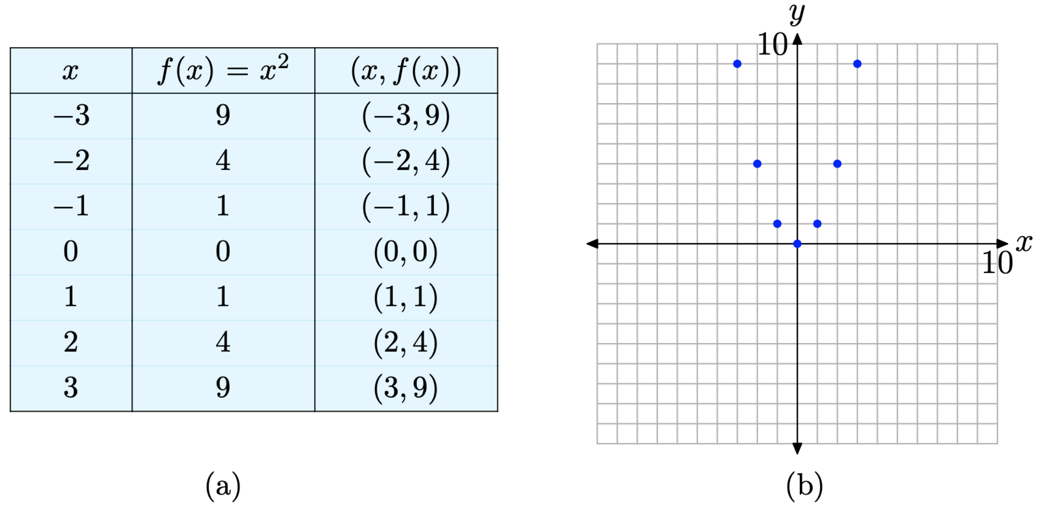
$WeChat550a7e418f62c4657b461ce068edd0e3.png$

Figure $\PageIndex{1}$. Plotting pairs satisfying the functional relationship defined by the equation $f(x)=x^{2}$.

The points we found appear to establish a pattern for the function behavior so we draw the graph by connecting the points. Since the domain is all real numbers, we draw arrows at the edge of the coordinate system to indicate the graphical pattern continues upward.

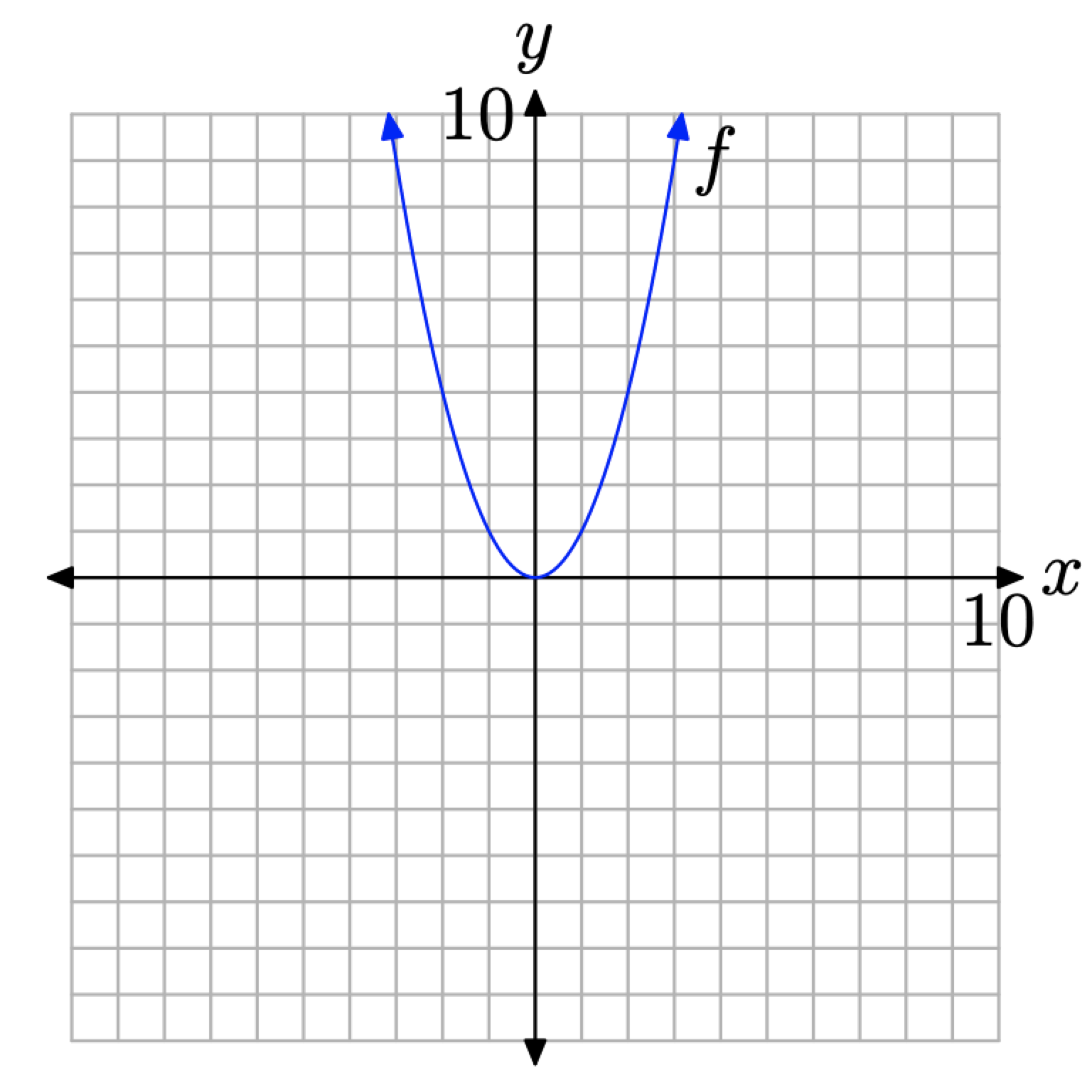
$WeChat8fc04a090466f5d15bb15909949fdb78.png$

Figure $\PageIndex{2}$. Plotting all pairs $(x, f(x))$ so that x is in the domain of f.

Strategy for Graphing by Hand Using Points

If a function is defined by an equation, you can create the graph of the function as follows.

Select several values of x in the domain of the function f.
Use the selected values of x to create a table of pairs (x, f(x)) that satisfy the equation that defines the function f.
Create a Cartesian coordinate system on a sheet of graph paper. Label and scale each axis, then plot the pairs (x, f(x)) from your table on your coordinate system.
If the plotted pairs (x, f(x)) provide enough of a pattern for you, make the “leap of faith” and plot all pairs that satisfy the equation defining f by drawing a graph on your coordinate system.
If your plotted pairs do not provide enough of a pattern to determine the final shape of the graph of f, then find more add more pairs and plot them. Continue in this manner until you are confident in the shape of the graph of f.

Let’s look at some more examples of graphing by hand.

Example $\PageIndex{1}$

Sketch the graph of the function defined by the equation $f(x)=x^{3}$.

Solution

We’ll start with x-values $-2,-1,0,1,$ and 2, then use the equation $f(x)=x^{3}$ to determine pairs (x, f(x)) (e.g., $f(-2)=(-2)^{3}=-8$). These are listed in the table in Figure $\PageIndex{3}$(a). We then plot the points from the table on a Cartesian coordinate system, as shown in Figure $\PageIndex{3}$(b).

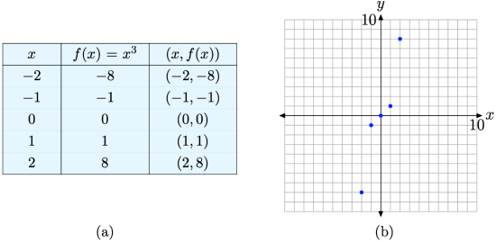
$WeChat4c93a6d748b5ef765b90768729e3a9d3.png$

Figure $\PageIndex{3}$. Plotting pairs (x, f(x)) defined by the equation $f(x)=x^{3}$.

We’re a bit unsure of the shape of the graph of f, so we’ll add a few more points to our table and plot them. This is shown in Figures $\PageIndex{4}$(a) and (b).

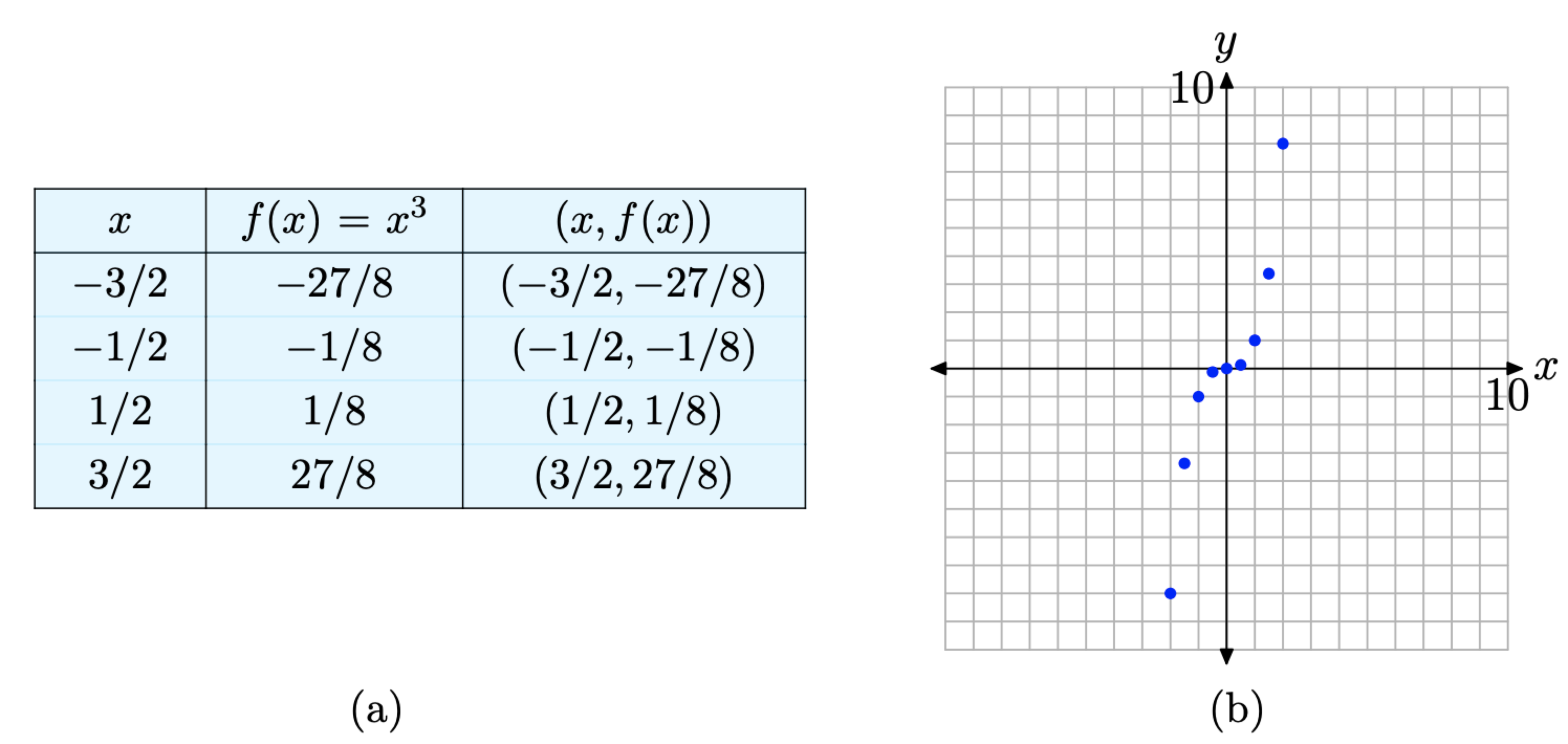
$WeChat6183b0cefb3c205270a88f8d8becc92c.png$

Figure $\PageIndex{4}$. Plotting additional pairs (x, f(x)) defined by the equation $f(x)=x^{3}$.

The additional pairs fill in the shape of f in Figure $\PageIndex{4}$(b) a bit better than those in Figure $\PageIndex{3}$(b), enough so that we’re confident enough to draw the final shape of the graph of $f(x)=x^{3}$ in Figure $\PageIndex{5}$.

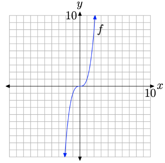
$WeChata87eff3a88c488120e43298cc85d2038.png$

Figure $\PageIndex{5}$. The final graph of $f(x)=x^{3}$.

Let’s look at another example.

Example $\PageIndex{2}$

Sketch the graph of $f(x)=\sqrt{x}$

Solution

Again, we’ll start by selecting several values of x in the domain of f. In this case, $f(x)=\sqrt{x}$, and it’s not possible to take the square root of a negative number. Also, if we’re creating a table of pairs by hand, it’s good strategy to select known squares. Thus, we’ll use x = 0, 1, 4, and 9 for starters.

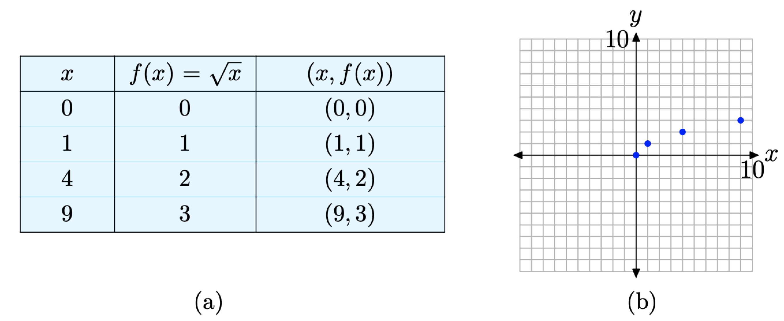
$WeChat0b62d9ccd5ee2cdf791e1dc0a664f343.png$

Figure $\PageIndex{6}$. Plotting pairs (x, f(x)) defined by the equation $f(x)=\sqrt{x}$.

Some might be ready to make a “leap of faith” based on these initial results. Others might want to use a calculator to compute decimal approximations for additional square roots. The resulting pairs are shown in the table in Figure $\PageIndex{7}$(a) and the additional pairs are plotted in Figure $\PageIndex{7}$(b).

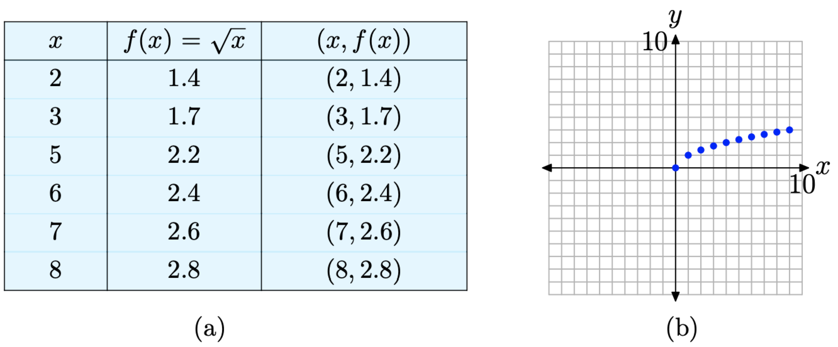
$WeChat926156d97f30e3a9b27cccc5f0c55c65.png$

Figure $\PageIndex{7}$ Plotting additional pairs (x, f(x)) defined by the equation $f(x)=\sqrt{x}$

The pattern in Figure $\PageIndex{7}$(b) is clear enough to complete the graph as shown in Figure $\PageIndex{8}$.

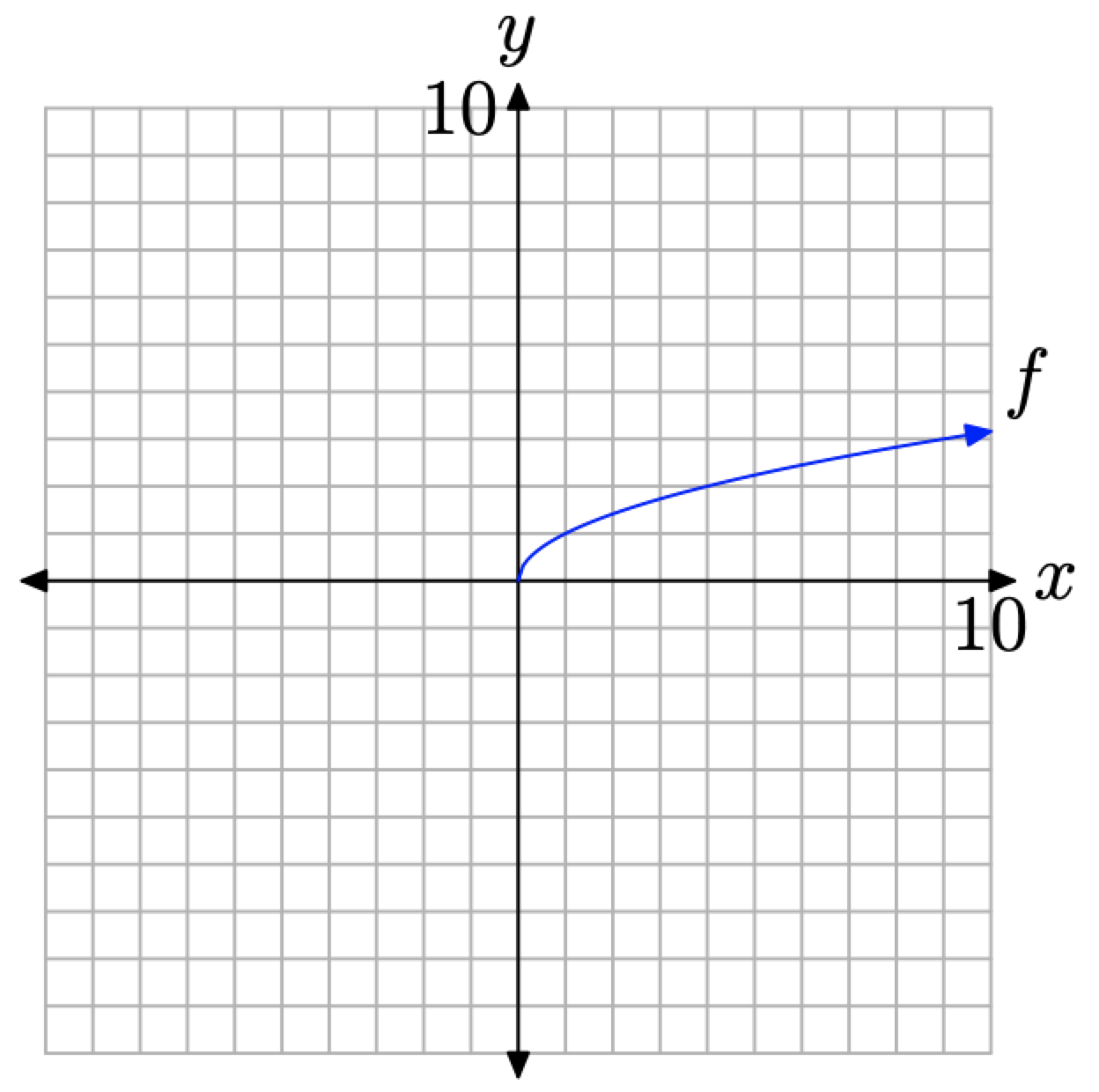
$WeChatfe79e2db6b46c5e0296c8557913e2a3c.png$

Figure $\PageIndex{8}$. The graph of f defined by the equation $f(x)=\sqrt{x}$.

Using a Graphing Calculator to Find Points and Graph Functions

The TABLE feature on your graphing calculator can be of immense help when creating tables of points that satisfy the equation defining the function f. Let’s look at an example

Example $\PageIndex{3}$

Sketch the graph of $f(x)=|x|$

Solution

Enter the function $f(x)=|x|$ in the $\mathrm{Y}=$ menu as follows.

Press the Y= button on your calculator. This will open the Y= menu as shown in Figure $\PageIndex{9}$(a). Use the arrow keys and the CLEAR button on your calculator to delete any existing functions.
Press the MATH button to open the menu shown in Figure $\PageIndex{9}$(b).
Press the right-arrow on your calculator to select the NUM submenu as shown in Figure $\PageIndex{9}$(c).
Select 1:abs(, then enter X and close the parentheses, as shown in Figure $\PageIndex{9}$(d).

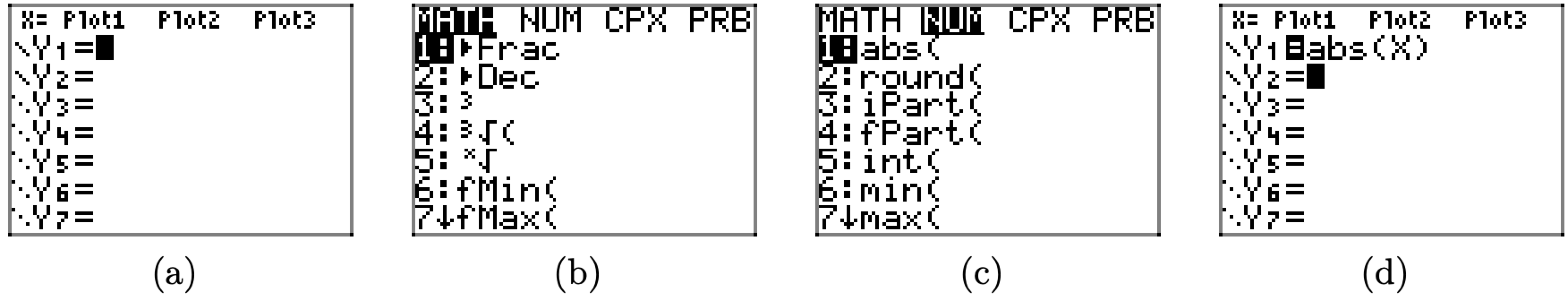
$WeChat12a410cf3fcce36778040dd1b2e2b6f7.png$

Figure $\PageIndex{9}$. Entering $f(x)=|x|$ in the $\mathrm{Y}=$ menu.

We will now use the TABLE feature of the graphing calculator to help create a table of pairs (x, f(x)) satisfying the equation $f(x) = |x|$. Proceed as follows.

Select 2nd TBLSET (i.e., push the 2nd button followed by TBLSET), which is located over the WINDOW button. Enter TblStart=-3, $\Delta \mathrm{Tb} 1=1$, and set the independent and dependent variables to Auto (this is done by highlighting Auto and pressing the Enter button), as shown in Figure $\PageIndex{10}$(a).
Press 2nd TABLE, which is located above the GRAPH button, to produce the table of pairs (x, f(x)) shown in Figure $\PageIndex{10}$(b).

We’ve plotted the pairs directly from the calculator onto a Cartesian coordinate system on graph paper in Figure $\PageIndex{10}$(c).

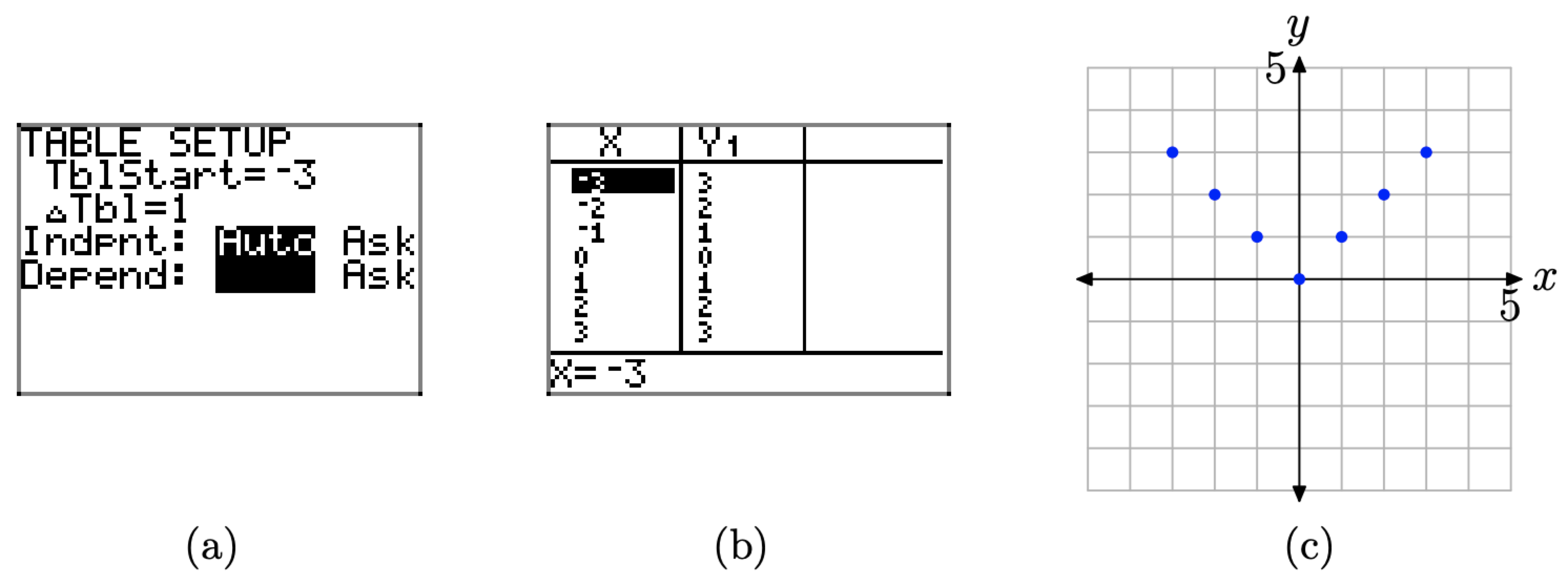
$WeChat16eb680e8ce839d8804a53f7e6b3b760.png$

Figure $\PageIndex{10}$. Creating a table with the TABLE feature of the graphing calculator.

We can have the graphing calculator draw the graph for us. Push the ZOOM button, then select 6:ZStandard (shown in Figure $\PageIndex{11}$(a)) to produce the graph shown in Figure $\PageIndex{11}$(b).

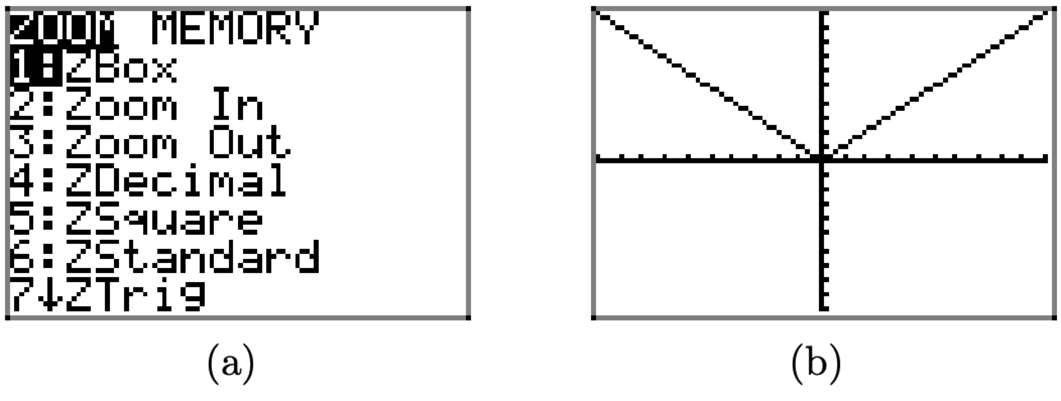
$WeChat12f1bbaa8809632c4b9bc777e6c5c21a.png$

Figure $\PageIndex{11}$. Creating the graph of $f(x) = |x|$ with the graphing calculator.

Note: The standard graphing calculator window, 6:ZStandard, is:\[-10 \leq {x} \leq {-10} \text{ and } -10 \leq {y} \leq {-10}\nonumber\]

The functions discussed so far are sometimes referred to as parent functions, basic functions, or tool box functions. They will be important later when we look at more efficient ways to graph functions.

Adjusting the Calculator Viewing Window

In Example $\PageIndex{3}$, we used the graphing calculator to draw the graph of the function defined by the equation $f(x) = |x|$. For the functions we’ve encountered thus far, drawing their graphs using the graphing calculator is pretty trivial. Simply enter the equation in the Y= menu, then press the ZOOM button and select 6:ZStandard. However, if the graph of a function doesn’t fit (or even appear) in the “standard” viewing window, it can be quite challenging to find optimal view settings so that the important features of the graph are visible.

Indeed, as one might not even know what “important” features to look for, setting the viewing window is usually highly subjective and experimental by nature. Let’s look at some examples.

Example $\PageIndex{4}$

Use a graphing calculator to sketch the graph of $f(x)=56-x-x^{2}$ using the window: Xmin = -15, Xmax = 15, Ymin = -100, Ymax = 100

Solution

First, start by entering the function in the Y= menu, as shown in Figure $\PageIndex{12}$(a). The caret ˆ on the keyboard is used for exponents. Press the ZOOM button and then select 6:ZStandard to produce the graph shown in Figure $\PageIndex{12}$(b).

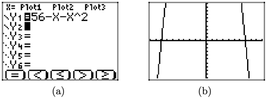
$WeChat4288a58fc63b28e68193246123f0b764.png$

Figure $\PageIndex{12}$. The graph of $f(x)=56-x-x^{2}$ in the “standard” viewing window.

To change the window, push the WINDOW button. Now, set Xmin = -15 and Xmax = 15. Xscl changes the units on the x-axis. If we want the tick marks on the scale to be 5 units, set Xscl = 5. Next, set Ymax = 100 and Ymin = -100. Since this is a wide interval, let's set tick marks on the y-axis every 10 units with Yscl = 10.

Push the GRAPH button to view the effects of these changes to the WINDOW parameters in Figure $\PageIndex{13}$(b).

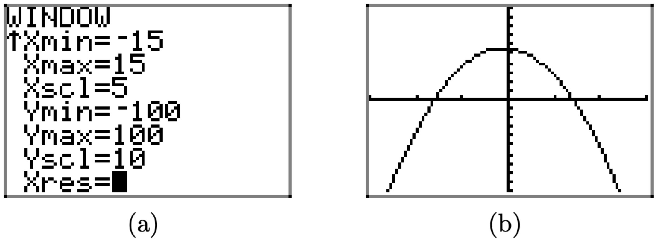
$WeChat8af13eafc532d408e1d74b79e582a9fb.png$

Figure $\PageIndex{13}$. Improving the WINDOW settings.

In the previous example, the window setting were provided. We can see in Figure $\PageIndex{12}$(b) and $\PageIndex{13}$(b) that different windows provide different visuals of the graph. We usually prefer to use window settings that show the "important features" of function. If one is just beginning to learn about the graphs of functions, how is one to determine what are good windows for viewing the “important features” of the graph? Unfortunately, the answer to this question is, “through experience.” Undoubtedly, this is a very frustrating phrase for readers to hear, but at least it’s truthful. The more graphs that you draw, the more you will learn how to look for “turning points,” “end-behavior,” “x- and y-intercepts,” and the like.

Legend for Graphing Calculator Window Parameters

The following explains each of the WINDOW parameters in Figure $\PageIndex{13}$(a).

Xmin is the x-value of left edge of viewing window

Xmax is the x-value of right edge of viewing window

Xscl is the x-axis tick increment

Ymin is the y-value of bottom edge of viewing window

Ymax is the y-value of top edge of viewing window

Yscl is the y-axis tick increment

Xres is a pixel setting for viewing. Most people leave this setting at 1

Note: If the Xmin $\geq{}$ Xmax, the calculator will not graph and it will give you an error message. Similiarly, this will also occur if Ymin $\geq{}$ Ymax

Determining If a Graph Represents a Function (Vertical Line Test)

As we have seen in some examples above, we can represent a function using a graph. Graphs display a great many input-output pairs in a small space. The visual information they provide often makes relationships easier to understand. By convention, graphs are typically constructed with the input values along the horizontal axis and the output values along the vertical axis.

The most common graphs name the input value $x$ and the output $y$, and we say $y$ is a function of $x$, or $y=f(x)$ when the function is named $f$. The graph of the function is the set of all points $(x,y)$ in the plane that satisfies the equation $y=f(x)$. If the function is defined for only a few input values, then the graph of the function is only a few points, where the x-coordinate of each point is an input value and the y-coordinate of each point is the corresponding output value. For example, the black dots on the graph in Figure $\PageIndex{10}$ tell us that $f(0)=2$ and $f(6)=1$. However, the set of all points $(x,y)$ satisfying $y=f(x)$ is a curve. The curve shown includes $(0,2)$ and $(6,1)$ because the curve passes through those points

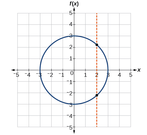
Figure $\PageIndex{14}$: Graph of a polynomial.

The vertical line test can be used to determine whether a graph represents a function of x. If we can draw any vertical line that intersects a graph more than once, then the graph does not define a function of x because a function has only one output value for each input value. See Figure $\PageIndex{15}$.

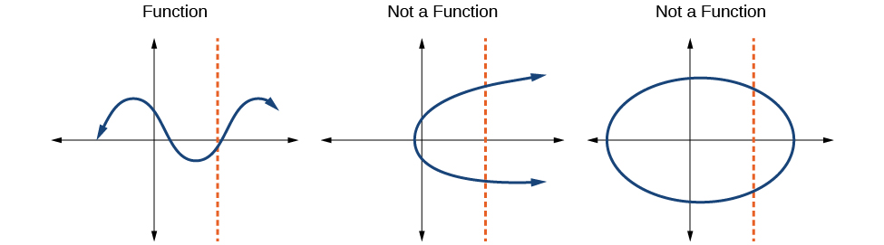
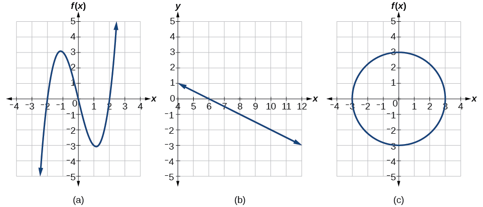
Figure $\PageIndex{15}$: Three graphs visually showing what is and is not a function.

Example $\PageIndex{5}$

Which of the graphs in Figure $\PageIndex{16}$ represent(s) a function $y=f(x)$?

Figure $\PageIndex{16}$: Graph of a polynomial (a), a downward-sloping line (b), and a circle (c).

Solution

If any vertical line intersects a graph more than once, the relation represented by the graph is not a function. Notice that any vertical line would pass through only one point of the two graphs shown in parts (a) and (b) of Figure $\PageIndex{16}$. From this we can conclude that these two graphs represent functions. The third graph does not represent a function because, at most x-values, a vertical line would intersect the graph at more than one point, as shown in Figure $\PageIndex{17}$.

Figure $\PageIndex{17}$: Graph of a circle.

You Try $\PageIndex{3}$

Does the graph in Figure $\PageIndex{18}$ represent a function?

[Absolute function f(x)=|x|.] — Figure $\PageIndex{18}$: Graph of absolute value function.

Answer: yes

Determining if an Equation Represents a Function

It is important to note that not every relationship expressed by an equation can also be expressed as a function with a formula. How do we then determine if an equation represents a function?

Example $\PageIndex{6}$

Does the equation $x^2+y^2=1$ represent a function of $x$? If so, express the relationship as a function $y=f(x)$.

Solution

First we subtract $x^2$ from both sides.

\[y^2=1−x^2 \nonumber\]

We now try to solve for $y$ in this equation.

\[y=\pm\sqrt{1−x^2} \nonumber\]

\[\text{so, }y=\sqrt{1−x^2}\;\text{and}\;y = −\sqrt{1−x^2} \nonumber\]

We get two outputs corresponding to the same input, so this relationship cannot be represented as a single function $y=f(x)$.

Note: Most graphing calculators are designed to only graph functions. To graph this equation in a graphing calculator properly, you must input both formulas into the calculator

Example: Y1=$\sqrt{1−x^2}$ and Y2=$−\sqrt{1−x^2} $

You Try $\PageIndex{2}$

Does the equation $x^3−8y=1$ represent a function of $x$? If so, express the relationship as a function $y=f(x)$.

Answer: $y=f(x)=\dfrac{x^3}{8}-\dfrac{1}{8}$ or $y=f(x)=\dfrac{x^3-1}{8}$

Q & A

Are there relationships expressed by an equation that do represent a function but which still cannot be represented by an algebraic formula?

Yes, this can happen. For example, given the equation $x=y+2^y$, if we want to express y as a function of x, there is no simple algebraic formula involving only $x$ that equals $y$. However, each $x$ does determine a unique value for $y$, and there are mathematical procedures by which $y$ can be found to any desired accuracy. In this case, we say that the equation gives an implicit (implied) rule for $y$ as a function of $x$, even though the formula cannot be written explicitly.

Evaluating Functions Using Graphs

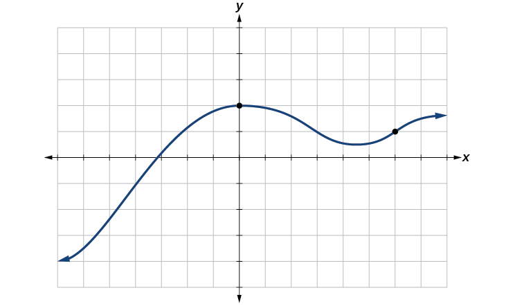
We know that the graph of f pictured in Figure $\PageIndex{19}$ is the graph of a function of x. We know this because no vertical line will cut the graph of f more than once.

We earlier defined the graph of f as the set of all ordered pairs $(x, f(x))$, so that x is in the domain of f. Consequently, if we select a point P on the graph of f, as in Figure $\PageIndex{19}$(a), we label the point P(x, f(x)). However, we can also label this point as $P(x, y)$ since y = f(x), as shown in Figure $\PageIndex{19}$(b).

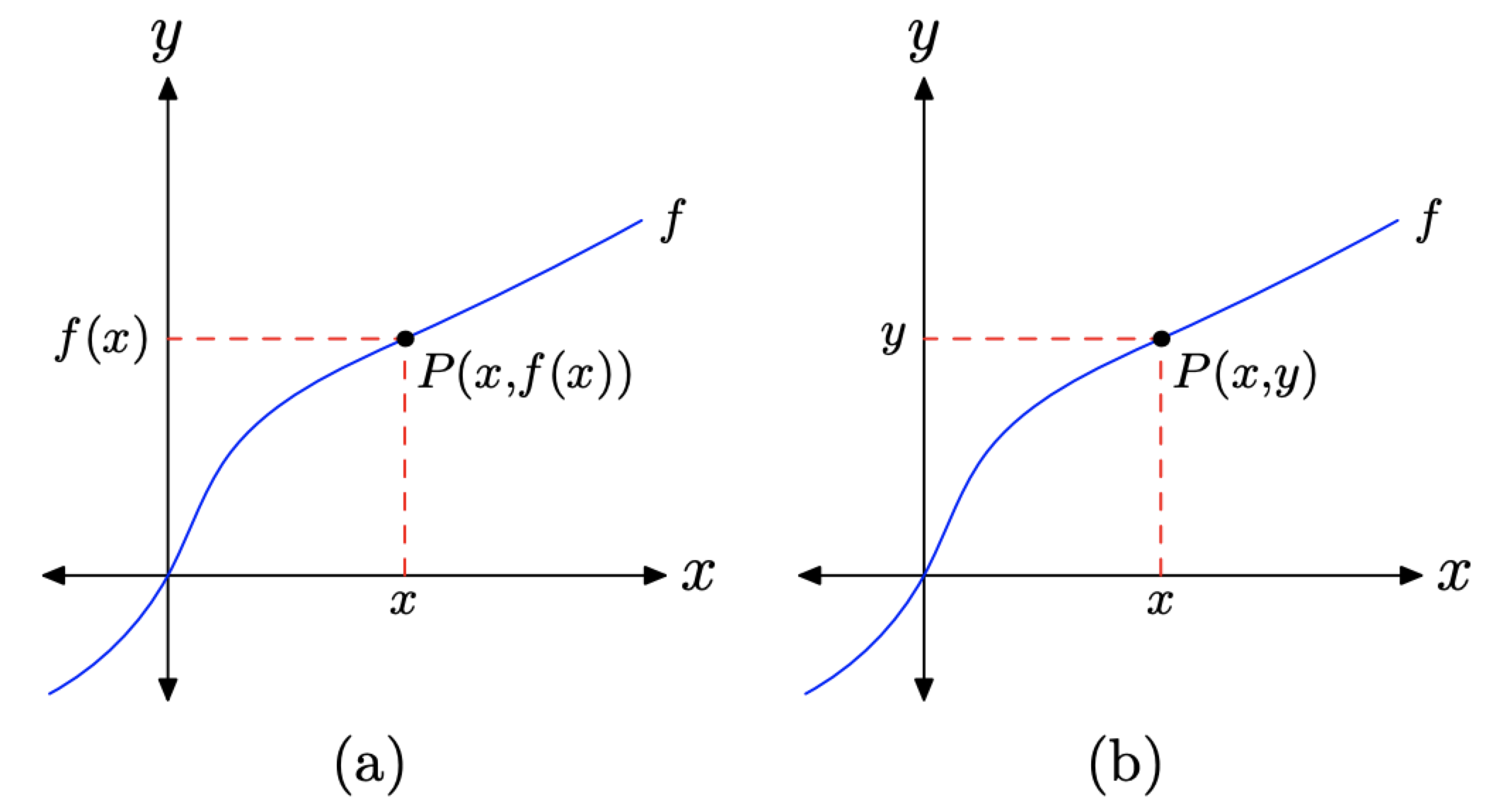
$WeChat9c7ca252bc58ace26d67a8b219bdb304.png$

Figure $\PageIndex{19}$. Reading the graph of a function.

Example $\PageIndex{7}$

Given the graph of a function f in Figure $\PageIndex{20}$(a), find f(4).

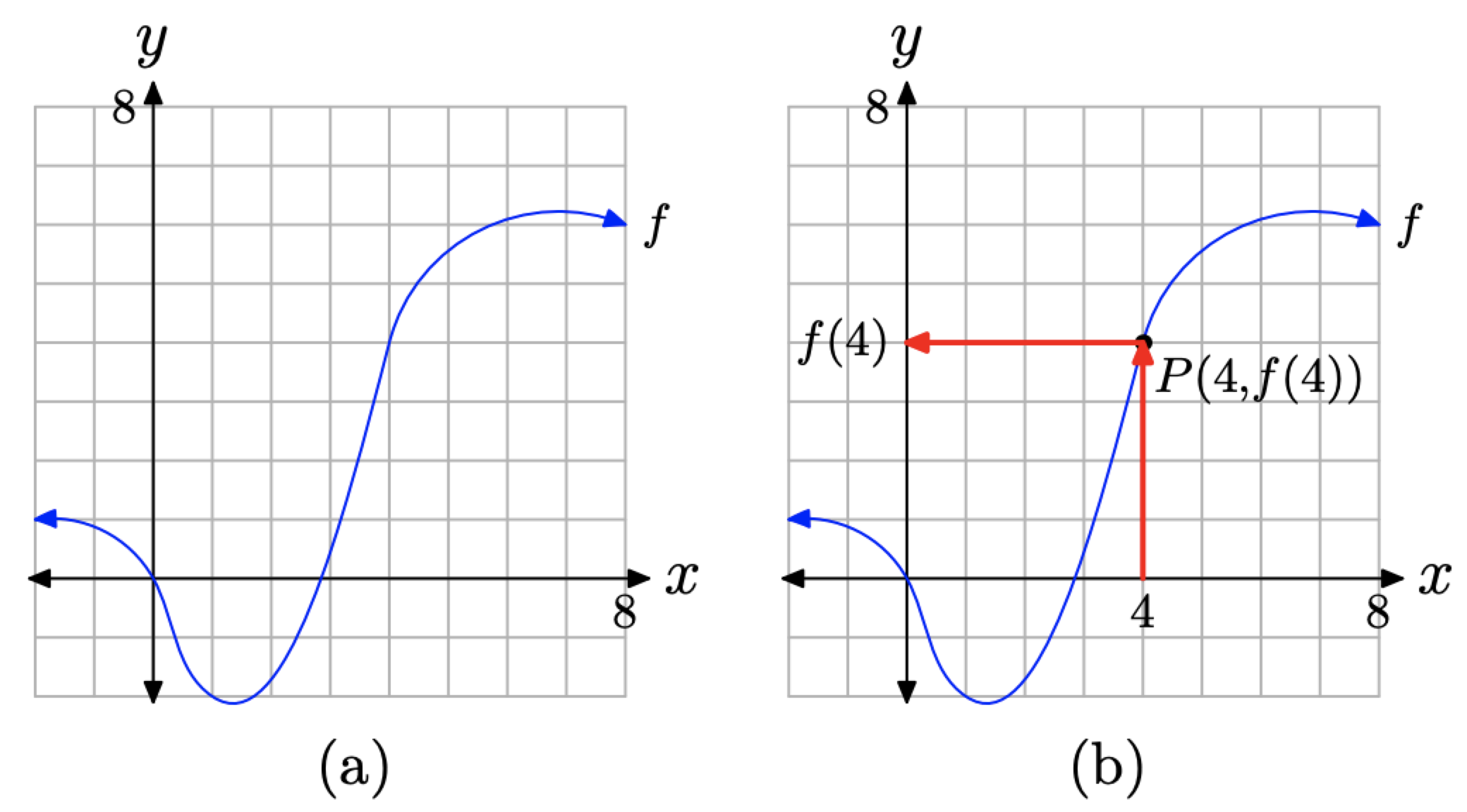
$WeChat7d2e5d9ef09b88527d9c0ed782222229.png$

Figure $\PageIndex{20}$. Finding the value of f(4).

Solution

Because f(4) represents the y-value that is paired with the x-value of 4, we first locate 4 on the x-axis, as shown in Figure $\PageIndex{20}$(b). We then draw a vertical arrow until we intercept the graph of f at the point P(4, f(4)). Finally, we draw a horizontal arrow from the point P until we intercept the y-axis. The projection of the point P onto the y-axis is the value of f(4).

Because we have a grid that shows a scale on each axis, we can approximate the value of f(4). It would appear that the y-value of point P is approximately 4. Thus, $f(4) \approx 4$.

Let’s reverse this process in another example.

Example $\PageIndex{8}$

Given the graph of a function, f, in Figure $\PageIndex{21}$(a), for what value of x does f(x) = −4?

Solution

This time, in the equation $f(x) = −4$, we’re given a y-value equal to −4. We must reverse the process used in the previous example. We first locate the y-value −4 on the y-axis, then draw a horizontal arrow until we intercept

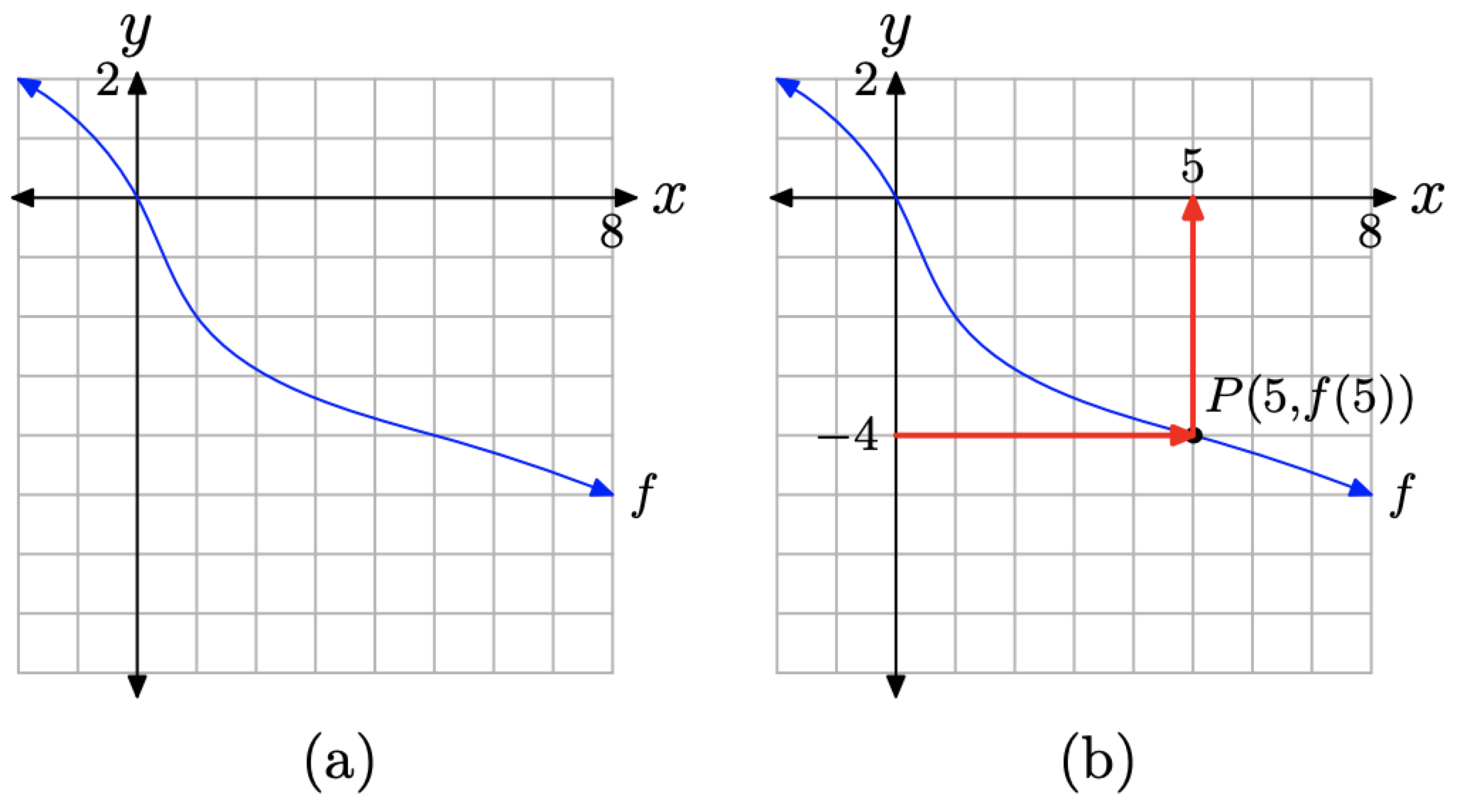
$WeChatd1ec47e296b2b9d4ccae38b2263430e3.png$

Figure $\PageIndex{21}$. Finding x so that $f(x) = −4$.

the graph of f at P, as shown in Figure $\PageIndex{21}$(b). Finally, we draw a vertical arrow from the point P until we intercept the x-axis. The projection of the point P onto the x-axis is the solution of $f(x) = −4$.

Because we have a grid that shows a scale on each axis, we can approximate the x-value of the point P. It seems that $x \approx 5$. Thus, we label the point P(5, f(5)), and the solution of $f(x) = −4$ is approximately $x \approx 5$.

This solution can easily be checked by computing f(5). Simply start with 5 on the x-axis, then reverse the order of the arrows shown in Figure (\PageIndex{21}\)(b). You should wind up at −4 on the y-axis, demonstrating that $f(5) \approx −4$.

Basic Functions

Earlier it was mentioned that there are some functions we commonly work with. These functions are commonly referred to as parent functions, basic functions, or tool box functions. We want to be familiar with these functions so let's take a moment to define what they are.

For the basic quadratic function $f(x)=x^2$, the domain is all real numbers since the horizontal extent of the graph is the whole real number line. Because the graph does not include any negative values for the range, the range is only nonnegative real numbers.

For the basic cubic function $f(x)=x^3$, the domain is all real numbers because the horizontal extent of the graph is the whole real number line. The same applies to the vertical extent of the graph, so the domain and range include all real numbers.

For the basic square root function $f(x)=\sqrt{x}$, we cannot take the square root of a negative real number, so the domain must be 0 or greater. The range also excludes negative numbers because the square root of a positive number $x$ is defined to be positive, even though the square of the negative number $−\sqrt{x}$ also gives us $x$.

$[Square root function f(x)=sqrt(x).]$
Figure $\PageIndex{24}$: Square root function $f(x)=\sqrt{x}$.

For the basic cube root function $f(x)=\sqrt[3]{x}$, the domain and range include all real numbers. Note that there is no problem taking a cube root, or any odd-integer root, of a negative number, and the resulting output is negative (it is an odd function).

[Cube root function f(x)=x^(1/3).] — Figure $\PageIndex{25}$: Cube root function $f(x)=\sqrt[3]{x}$.

For the basic absolute value function $f(x)=|x|$, there is no restriction on $x$. However, because absolute value is defined as a distance from 0, the output can only be greater than or equal to 0.

All the basic functions listed above have a point at (0,0) and (1,1). This will be useful for later.

Graphing Piecewise Functions

Previously, we learned how to evaluate piecewise defined functions. Next, let's focus on how to graph them.

Given a piecewise function, sketch a graph.

Indicate on the x-axis the boundaries defined by the intervals on each piece of the domain.
For each piece of the domain, graph on that interval using the corresponding equation pertaining to that piece. Do not graph two functions over one interval because it would violate the criteria of a function.

Note: It is important to not just plot some points when graphing piecewise functions.

Example $\PageIndex{9}$

Sketch a graph of the function.

\[f(x)= \begin{cases} x^2 & \text{if $x \leq 1$} \\ 3 &\text{if $1<x\leq2$} \\ x &\text{if $x>2$} \end{cases} \nonumber \]

Solution

Each of the component functions is from our library of toolkit functions, so we know their shapes. We can imagine graphing each function and then limiting the graph to the piece we need for the indicated domain of the piecewise function we are graphing. At the endpoints of the domain interval, draw open circles to indicate where the endpoint is not included because of a less-than or greater-than inequality; we draw a closed circle where the endpoint is included because of a less-than-or-equal-to or greater-than-or-equal-to inequality.

Figure $\PageIndex{27}$ shows the three components of the piecewise function graphed on separate coordinate systems.

$[Graph of each part of the piece-wise function f(x)]$
Figure $\PageIndex{27}$: Graph of each part of the piece-wise function f(x)

(a)$ f(x)=x^2$ if $x≤1$; (b) $f(x)=3$ if $1< x≤2$; (c) $f(x)=x$ if $x>2$

Now that we have sketched each piece individually, we then combine them in the same coordinate plane to form the graph of the piecewise function. See Figure $\PageIndex{28}$.

[Graph of the entire function.] — Figure $\PageIndex{28}$: Graph of the entire function.

Analysis

Note that the graph does pass the vertical line test even at $x=1$ and $x=2$ because the points $(1,3)$ and $(2,2)$ are not part of the graph of the function, though $(1,1)$ and $(2, 3)$ are.

You Try $\PageIndex{10}$

Graph the following piecewise function.

\[f(x)= \begin{cases} x^3 & \text{if $x < -1$} \\ -2 &\text{if $-1<x<4$} \\ \sqrt{x} &\text{if $x>4$} \end{cases} \nonumber \]

Answer: $[Graph of f(x).]$
Figure $\PageIndex{29}$

Template:ContribArnold

Search

Strategy for Graphing by Hand Using Points

Example \(\PageIndex{1}\)

Example \(\PageIndex{2}\)

Example \(\PageIndex{3}\)

Example \(\PageIndex{4}\)

Legend for Graphing Calculator Window Parameters

Example \(\PageIndex{5}\)

You Try \(\PageIndex{3}\)

Example \(\PageIndex{6}\)

You Try \(\PageIndex{2}\)

Q & A

Example \(\PageIndex{7}\)

Example \(\PageIndex{8}\)

Example \(\PageIndex{9}\)

You Try \(\PageIndex{10}\)