2.6: Average Rate of Change
- Page ID
- 126511

- Find the average rate of change of a function.
Since functions represent how an output quantity varies with an input quantity, it is natural to ask about the rate at which the values of the function are changing. For example, the function \(C(t)\) below gives the average cost, in dollars, of a gallon of gasoline \(t\) years after 2000.
| \(t\) | 2 | 3 | 4 | 5 | 6 | 7 | 8 | 9 |
|---|---|---|---|---|---|---|---|---|
| \(C(t)\) | 1.47 | 1.69 | 1.94 | 2.30 | 2.51 | 2.64 | 3.01 | 2.14 |
If we were interested in how the gas prices had changed between 2002 and 2009, we could compute that the cost per gallon had increased from $1.47 to $2.14, an increase of $0.67. While this is interesting, it might be more useful to look at how much the price changed per year. You are probably noticing that the price didn’t change the same amount each year, so we would be finding the average rate of change over a specified amount of time.
The gas price increased by $0.67 from 2002 to 2009, over 7 years, for an average of \(\dfrac{\$ 0.67}{7years} \approx 0.096\) dollars per year. On average, the price of gas increased by about 9.6 cents each year.
A rate of change describes how the output quantity changes in relation to the input quantity. The units on a rate of change are output units per input units.
Some other examples of rates of change would be quantities like:
- A population of rats increases by 40 rats per week
- A barista earns $9 per hour (dollars per hour)
- A farmer plants 60,000 onions per acre
- A car can drive 27 miles per gallon
- A population of grey whales decreases by 8 whales per year
- The amount of money in your college account decreases by $4,000 per quarter
The average rate of change between two input values is the total change of the function values (output values) divided by the change in the input values.
\[\text{Average rate of change} = \dfrac{\text{Change in Output}}{\text{Change in Input}} = \dfrac{\Delta y}{\Delta x} =\dfrac{y_{2} -y_{1} }{x_{2} -x_{1} }\nonumber\]
Using the cost-of-gas function from earlier, find the average rate of change between 2007 and 2009.
Solution
From the table, in 2007 the cost of gas was $2.64. In 2009 the cost was $2.14.
The input (years) has changed by 2. The output has changed by $2.14 - $2.64 = -0.50.
The average rate of change is then \(\dfrac{-\$ 0.50}{2years}\) = -0.25 dollars per year
Using the same cost-of-gas function, find the average rate of change between 2003 and 2008
- Answer
-
\(\dfrac{$3.01 - $1.69}{5\ years} = \dfrac{$1.32}{5\ years} = 0.264\) dollars per year.
Notice that in the last example the change of output was negative since the output value of the function had decreased. Correspondingly, the average rate of change is negative.
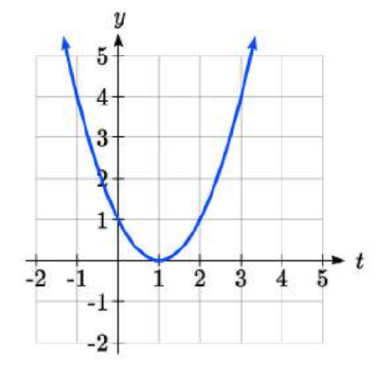
Given the function \(g(t)\) shown below in Figure \(\PageIndex{1}\), find the average rate of change on the interval [0, 3].
Solution
At t = 0, the graph shows \(g(0) = 1\)
At t = 3, the graph shows \(g(3) = 4\)
The output has changed by 3 while the input has changed by 3, giving an average rate of change of:
\[\dfrac{4-1}{3-0} =\dfrac{3}{3} =1\nonumber \]
On a road trip, after picking up your friend who lives 10 miles away, you decide to record your distance from home over time. Find your average speed over the first 6 hours.
| \(t\) (hours) | 0 | 1 | 2 | 3 | 4 | 5 | 6 | 7 |
|---|---|---|---|---|---|---|---|---|
| \(D(t)\) (miles) | 10 | 55 | 90 | 153 | 214 | 240 | 292 | 300 |
Solution
Here, your average speed is the average rate of change.
You traveled 282 miles in 6 hours, for an average speed of
\[\dfrac{292-10}{6-0} =\dfrac{282}{6}= 47\text{ miles per hour}\nonumber\]
We can more formally state the average rate of change calculation using function notation.
Given a function \(f(x)\), the average rate of change on the interval [a, b] is
\[\text{Average rate of change} = \dfrac{\text{Change of Output}}{\text{Change of Input}} =\dfrac{f(b)-f(a)}{b-a} \label{avgratefunction}\nonumber\]
Compute the average rate of change of \(f(x)=x^{2} -\dfrac{1}{x}\) on the interval [2, 4].
Solution
We can start by computing the function values at each endpoint of the interval
\[f(2)=2^{2} -\dfrac{1}{2} =4-\dfrac{1}{2} =\dfrac{7}{2} \nonumber\]
\[f(4)=4^{2} -\dfrac{1}{4} =16-\dfrac{1}{4} =\dfrac{63}{4} \nonumber\]
Now computing the average rate of change
\[\text{Average rate of change} = \dfrac{f(4) - f(2)}{4 - 2} =\dfrac{\dfrac{63}{4} -\dfrac{7}{2} }{4-2} =\dfrac{\dfrac{49}{4} }{2} = \dfrac{49}{8} \nonumber\]
Find the average rate of change of \(f(x) = x - 2\sqrt{x}\) on the interval [1, 9].
- Answer
-
Average rate of change = \(\dfrac{f(9) - f(1)}{9 - 1} = \dfrac{(9 - 2\sqrt{9}) - (1 - 2\sqrt{1})}{9 - 1} = \dfrac{(3) - (-1)}{9 - 1} = \dfrac{4}{8} = \dfrac{1}{2}\)
The magnetic force \(F\), measured in Newtons, between two magnets is related to the distance between the magnets \(d\), in centimeters, by the formula \(F(d)=\dfrac{2}{d^{2} }\). Find the average rate of change of force if the distance between the magnets is increased from 2 cm to 6 cm.
Solution
We are computing the average rate of change of \(F(d)=\dfrac{2}{d^{2} }\) on the interval [2, 6].
Average rate of change = \(\dfrac{F(6) - F(2)}{6 - 2}\)
Evaluating the function
\[\dfrac{F(6)-F(2)}{6-2} =\nonumber \]
\[= \dfrac{\dfrac{2}{6^{2} } -\dfrac{2}{2^{2} } }{6-2}\nonumber \] Simplifying
\[= \dfrac{\dfrac{2}{36} -\dfrac{2}{4} }{4}\nonumber \] Combining the numerator terms
\[= \dfrac{\dfrac{-16}{36} }{4}\nonumber \] Simplifying further
\[= \dfrac{-1}{9}\nonumber \] Newtons per centimeter
This tells us the magnetic force decreases, on average, by 1/9 Newtons per centimeter over this interval.
Find the average rate of change of \(g(t)=t^{2} +3t+1\)on the interval \([0, a]\). Your answer will be an expression involving a.
Solution
Using the average rate of change formula
\[\dfrac{g(a)-g(0)}{a-0}\nonumber\]
Evaluating the function
\[\dfrac{(a^{2} +3a+1)-(0^{2} +3(0)+1)}{a-0}\nonumber\]
Simplifying
\[\dfrac{a^{2} +3a+1-1}{a}\nonumber\]
Simplifying further, and factoring
\[\dfrac{a(a+3)}{a}\nonumber\]
Cancelling the common factor \(a\)
\[a+3\nonumber\]
This result tells us the average rate of change between t = 0 and any other point t = a. For example, on the interval [0, 5], the average rate of change would be 5+3 = 8.
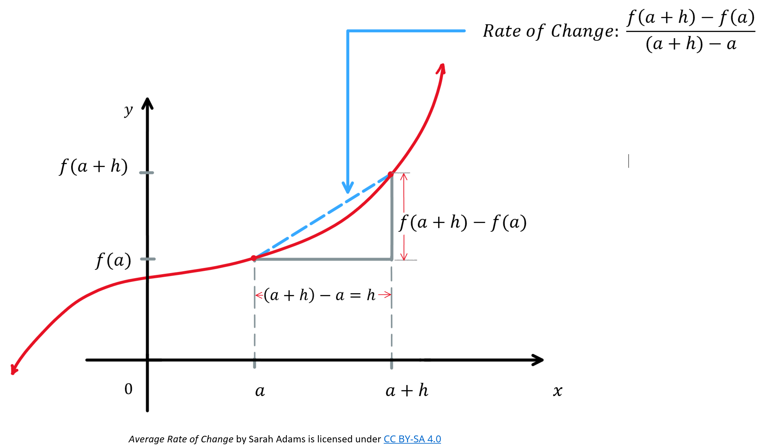
Find the average rate of change of \(f(x)=x^{3} +2\) on the interval \([a,a+h]\).
- Answer
-
\[\dfrac{f(a + h) - f(a)}{(a + h) - a} = \dfrac{((a + h)^3 + 2) - (a^3 + 2)}{h} = \dfrac{a^3 + 3a^2h + 3ah^2 + h^3 + 2 - a^3 - 2}{h} = \dfrac{3a^2h + 3ah^2 + h^3}{h} = \dfrac{h(3a^2 + 3ah + h^2)}{h} = 3a^2 + 3ah + h^2\nonumber\]
Do remember to watch out for common arithmetic errors: \((a+h)^3 \neq{a^3+h^3}\).
Instead, expand the product to help ensure the multiplication is done correctly: \((a+h)^3 = (a+h)(a+h)(a+h)\)
You may be wondering why we would want to find the average rate of change on an interval such as \([a,a+h]\). The value "a" represents an arbitrary x-coordinate for a point. The value "a+h" represents another arbitrary x-coordinate of another point. The value "h" represents the horizontal distance between these two points. The average rate of change on this interval, \([a,a+h]\), is \[\dfrac{f(a + h) - f(a)}{(a + h) - a}\nonumber\] which is visually the slope of a secant line passing through these two points on the graph of the function, as shown in Figure \(\PageIndex{2}\) below. In calculus, you will investigate what happens to the slope of this secant line as you change the distance "h" between the two points. By shrinking this distance we can describe instantaneous rate of change which is a very useful topic in many real-life situations. Stay tuned for more about this in your future calculus course!